How To Create A Drop Down List In Google Sheets

Introduction

Welcome to our step-by-step guide on how to create a drop-down list in Google Sheets. If you’ve ever wanted to streamline data entry or ensure consistency when inputting information, a drop-down list can be a valuable tool. By limiting the options to a predefined list, you can avoid errors and enhance the efficiency of your spreadsheet.

Google Sheets is a powerful online spreadsheet application that offers a wide range of features and functionalities. Creating a drop-down list might seem intimidating at first, but rest assured, it’s a straightforward process that can be done in just a few simple steps. Whether you’re a beginner or an experienced Sheets user, this guide will walk you through the process, ensuring that you can easily implement drop-down lists in your own projects.

By the end of this tutorial, you’ll have the knowledge and confidence to create custom drop-down lists that suit your specific needs. So, let’s jump right in and get started!

Step 1: Open Google Sheets

The first step in creating a drop-down list in Google Sheets is to open the Sheets application. If you don’t already have a Google account, you’ll need to create one in order to access Google Sheets. Once you’re logged in, follow the steps below:

1. Go to the Google Sheets homepage by typing https://sheets.google.com into your web browser’s address bar and pressing Enter.
2. If you already have a spreadsheet that you want to add a drop-down list to, open it by clicking on the file name in your Google Drive or by navigating to the “Sheets” section and finding your file.
3. Alternatively, you can create a new spreadsheet by clicking on the “+ New” button located at the top left corner of the page and selecting “Google Sheets” from the dropdown menu.

Once you have opened Google Sheets and selected the desired spreadsheet, you’re ready to proceed to the next step: selecting the cell range where you want to create the drop-down list.

Step 2: Select the Cell Range

After opening your Google Sheets spreadsheet, the next step in creating a drop-down list is to select the cell range where you want the drop-down list to appear. The cell range defines the area where the drop-down list will be visible and can be easily adjusted based on your specific needs. Follow the instructions below to select the desired cell range:

1. Click on the first cell in the range where you want the drop-down list to start.
2. Drag your cursor across the cells to select the entire range. You can select a single column, a single row, or a combination of multiple rows and columns.
3. Alternatively, you can manually input the cell range by typing it into the address bar located at the top left corner of the Sheets application. For example, if you want the drop-down list to appear in cells A1 to A10, you would type “A1:A10”.

It’s important to ensure that the selected cell range is appropriate for your particular use case. Make sure that the range includes enough cells to accommodate the options you plan to enter in the drop-down list. Once you have selected the desired cell range, you’re ready to move on to the next step: accessing the “Data” menu.

Step 3: Go to “Data” in the Menu

After selecting the cell range where you want to create the drop-down list, the next step is to navigate to the “Data” menu in Google Sheets. The “Data” menu contains a variety of options for managing and manipulating your data, including the ability to add data validation and create drop-down lists. Here’s how you can access the “Data” menu:

1. Look for the menu bar at the top of the Google Sheets application.
2. Click on the “Data” option in the menu. This will display a dropdown menu with various data-related options.

By clicking on the “Data” option, a menu will appear, allowing you to access additional data-related functionalities. This menu is where you’ll find the option to add data validation, which is necessary for creating a drop-down list. In the next step, we’ll explore how to access the “Data validation” option and begin setting up our drop-down list criteria.

Step 4: Click on “Data validation”

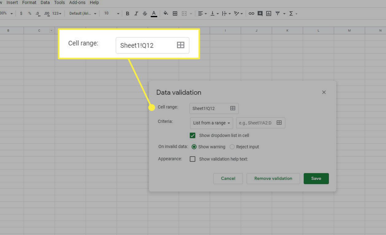
Once you have accessed the “Data” menu in Google Sheets, the next step is to click on the “Data validation” option. This will open a dialog box where you can specify the criteria for your drop-down list. Follow the instructions below to proceed:

1. Click on the “Data validation” option in the “Data” menu. A dialog box titled “Data validation” will appear.
2. In the “Data validation” dialog box, you’ll see various settings that you can customize to define the behavior and appearance of your drop-down list.
3. If there is already data validation applied to the selected cell range, you might see the existing settings pre-populated in the dialog box. You can modify these settings or start from scratch.

Clicking on “Data validation” is a crucial step in creating your drop-down list. This is where you’ll define the rules and conditions for what can be entered into the selected cell range. In the next step, we’ll explore how to set the criteria specifically for creating a list-based drop-down menu.

Step 5: Set the Criteria

Once you have opened the “Data validation” dialog box in Google Sheets, the next step is to set the criteria for your drop-down list. This is where you specify the rules and limitations for the data that can be entered into the selected cell range. Follow the instructions below to set the criteria:

1. In the “Data validation” dialog box, you’ll see a section labeled “Criteria”. This section allows you to choose the type of data validation you want to apply to the selected cell range.
2. From the “Criteria” drop-down menu, select the option that says “List from a range”. This will enable the list-based drop-down menu.
3. Once you select “List from a range”, additional fields will appear where you can specify the range of cells that contain the options for your drop-down list. This range should include all the options you want to appear in the drop-down menu.
4. If your list is located on a different sheet within the same spreadsheet, be sure to include the sheet name followed by an exclamation mark (!) before the cell range. For example, if your list is on Sheet2 in cells A1 to A5, you would enter: Sheet2!A1:A5

Setting the criteria is a crucial step in creating your drop-down list. It allows you to define the options that will appear in the drop-down menu and restricts the data that can be entered into the selected cell range. In the next step, we’ll explore how to customize the behavior and appearance of your drop-down list.

Step 6: Choose “List from a range”

After setting the criteria for your drop-down list in Google Sheets, the next step is to choose the option “List from a range” within the “Data validation” dialog box. This option allows you to specify a range of cells that contains the options you want to appear in the drop-down menu. Follow the instructions below to proceed:

1. In the “Criteria” section of the “Data validation” dialog box, click on the drop-down menu.
2. From the options provided, select the choice that says “List from a range”. This tells Google Sheets that you want to create a drop-down list based on a specific range of cells.
3. Once you have selected “List from a range”, additional fields will appear where you can enter the cell range that contains your list of options.
4. Specify the range by typing the cell references directly into the field or by clicking on the small grid icon and selecting the range using the visual interface.

Choosing “List from a range” is a crucial step in creating your drop-down list. This option allows you to define the range of cells that contains the options you want to appear in the drop-down menu. In the next step, we’ll cover how to select the specific range for your drop-down list.

Step 7: Select the Range for the List

After choosing the “List from a range” option in the “Data validation” dialog box, the next step is to select the range of cells that contains the options for your drop-down list. This range defines the values that will be available in the drop-down menu. Follow the instructions below to select the range:

1. Within the “Data validation” dialog box, look for the field where you can specify the range for your drop-down list.
2. Click on the field and either type in the cell range manually or click on the small grid icon for a visual interface to select the range.
3. Ensure that the range you specify includes all the cells that contain the options you want to appear in the drop-down menu.
4. If your list is on a different sheet within the same spreadsheet, be sure to include the sheet name followed by an exclamation mark (!) before the cell range.

Selecting the range for the drop-down list is an essential step in ensuring that the correct options are available in the drop-down menu. This range determines the values that users can choose from when entering data into the selected cell range. In the next step, we’ll explore how to customize the behavior and appearance of your drop-down list.

Step 8: Customize the Behavior and Appearance

After selecting the range for your drop-down list in Google Sheets, the next step is to customize its behavior and appearance. The “Data validation” dialog box provides several options that allow you to control how the drop-down list behaves and how it appears to users. Follow the instructions below to customize the behavior and appearance:

1. Within the “Data validation” dialog box, you’ll find various sections that allow you to customize the drop-down list.
2. Options such as “Show dropdown list in cell” allow you to choose whether the drop-down arrow should be visible directly in the cell or as a separate dropdown button.
3. You can also determine whether users can enter values outside of the list and whether the list should display as an error message or a warning if an invalid entry is made.
4. Additionally, you can customize the appearance of the drop-down list by changing the font, font size, and cell background color.

Customizing the behavior and appearance of your drop-down list allows you to tailor it to your specific needs and preferences. You can control how the list interacts with users and ensure that it fits seamlessly into your spreadsheet design. Once you have customized the behavior and appearance, the next step is to apply the data validation to your selected cell range.

Step 9: Apply the Data Validation

After customizing the behavior and appearance of your drop-down list in Google Sheets, the next step is to apply the data validation to the selected cell range. This ensures that the drop-down list is implemented and enforced within the spreadsheet. Follow the instructions below to apply the data validation:

1. Within the “Data validation” dialog box, review all the settings and options you have chosen to ensure they align with your intended drop-down list behavior and appearance.
2. Once you are satisfied with the customization, click on the “Save” or “Apply” button to apply the data validation to the selected cell range.
3. The dialog box will close, and you will see the drop-down list in the selected cell range. The drop-down arrow or button will indicate that a drop-down list has been created.

Applying the data validation is the final step in creating your drop-down list. It activates the list and ensures that the chosen rules and limitations are enforced when entering data into the selected cell range. With the data validation applied, you can now begin using and testing your drop-down list. In the next step, we’ll cover how to test the functionality of your drop-down list.

Step 10: Test the Drop Down List

Now that you have created and applied the data validation for your drop-down list in Google Sheets, it’s time to test its functionality. Testing the drop-down list ensures that it behaves as expected and allows you to verify that the options are displayed correctly. Follow the steps below to test the drop-down list:

1. Select one of the cells within the range where you applied the data validation for the drop-down list.
2. Click on the drop-down arrow or button in the cell to open the drop-down menu.
3. Verify that the options you specified in the data validation settings are displayed in the drop-down list.
4. Try selecting different options from the drop-down list to see how the selected value appears in the cell.
5. Ensure that you cannot enter values manually that are not part of the drop-down list.

Testing the drop-down list allows you to ensure that it works correctly and that the options are displayed as intended. It also provides an opportunity to validate that the data validation rules are correctly enforced, preventing any invalid entries. By taking the time to thoroughly test the drop-down list, you can confidently use it in your spreadsheet to streamline data entry and improve data consistency.

Conclusion

Creating a drop-down list in Google Sheets is a simple yet powerful way to enhance data entry and ensure consistency within your spreadsheets. By following the step-by-step guide outlined above, you can easily implement drop-down lists and customize them to fit your specific needs.

Starting with opening Google Sheets and selecting the cell range, you learned how to access the “Data” menu and click on “Data validation” to set the criteria for your drop-down list. You then chose the “List from a range” option and selected the range of cells containing the options for your list. Customizing the behavior and appearance of the drop-down list allowed you to tailor it to your preferences.

With the data validation settings in place, you applied the validation to the selected cell range and confirmed the functionality of the drop-down list by testing it. Testing ensured that the drop-down list displayed the correct options and prevented any invalid entries.

By incorporating drop-down lists into your Google Sheets, you can streamline data entry, reduce errors, and improve data consistency. Whether you’re managing inventory, tracking expenses, or collaborating on a project, drop-down lists can significantly enhance the efficiency and accuracy of your spreadsheets.

Now that you have the knowledge and skills to create drop-down lists in Google Sheets, feel free to explore the various possibilities and incorporate them into your own projects. Get creative and make the most out of this powerful feature!