How To Make Alternating Colors In Google Sheets

Introduction

When working with Google Sheets, it’s not uncommon to have large amounts of data that can be overwhelming to look at. To make it easier to read and analyze, one useful technique is to apply alternating colors to rows or columns. Alternating colors can help visually separate data and make it more distinct, allowing you to quickly identify patterns or trends.

In this article, we will guide you through the steps to make alternating colors in Google Sheets. Whether you’re organizing financial information, tracking project progress, or creating a simple list, applying alternating colors can enhance the readability and visual appeal of your spreadsheets.

By using this technique, you can create a clear and structured layout for your data, making it easier to navigate and interpret. Plus, with the flexibility to choose from a variety of color schemes, you can customize the appearance of your spreadsheet to suit your preferences or to match the branding of your project.

Let’s dive into the step-by-step process of creating alternating colors in Google Sheets so that you can arrange your data in a visually appealing and organized way.

Step 1: Access Google Sheets

To begin, you will need to access Google Sheets, which is a cloud-based spreadsheet tool offered by Google. Since Google Sheets is a web-based application, you can access it directly from your web browser without needing to download or install any software.

To access Google Sheets, follow these simple steps:

1. Open your preferred web browser. Google Sheets is compatible with popular web browsers such as Google Chrome, Mozilla Firefox, Safari, and Microsoft Edge.
2. Type “Google Sheets” in the search bar or directly enter the URL https://www.google.com/sheets.
3. If you already have a Google account, click on the “Sign in” button located at the top right corner of the page. Enter your email address and password to sign in.
4. If you don’t have a Google account, click on the “Create account” button and follow the on-screen instructions to create a new Google account. Having a Google account will give you access to various Google services, including Google Sheets.
5. Once you are signed in, you will be redirected to the Google Sheets homepage, where you can create or open existing spreadsheets.

Now that you have successfully accessed Google Sheets, you are ready to create a new spreadsheet or open an existing one. Let’s move on to the next step to get started with applying alternating colors to your data.

Step 2: Open a new or existing spreadsheet

Once you have accessed Google Sheets, you have the option to either open a new spreadsheet or open an existing one. Opening a new spreadsheet allows you to start from scratch, while opening an existing one lets you apply alternating colors to an already populated sheet.

Here’s how you can open a new or existing spreadsheet:

1. On the Google Sheets homepage, you will see a “+ New” button located in the top left corner. Click on it to open a drop-down menu.
2. From the drop-down menu, select “Blank spreadsheet” to open a new, empty sheet.
3. If you want to open an existing spreadsheet, click on “Folder” in the drop-down menu to access sheets saved in your Google Drive. You can browse through your folders to locate and open the desired spreadsheet.
4. If you already have a spreadsheet open, you can switch between different sheets by clicking on the name of the sheet located at the bottom of the window.

Whether you choose to open a new or existing sheet, make sure you have the spreadsheet in front of you before proceeding to the next step. If you are working on an existing sheet, ensure that the data you want to apply alternating colors to is visible on the screen.

Now that you have a blank or existing spreadsheet open, let’s move on to the next step to select the range of cells you want to apply alternating colors to.

Step 3: Select the range of cells you want to apply alternating colors to

Before you can apply alternating colors to your data in Google Sheets, you need to select the range of cells that you want to format. This step allows you to specify the area of your spreadsheet where the alternating colors will be applied.

To select the range of cells, follow these steps:

1. Click on the cell from which you want to start the selection. This will be the top-left cell of the range you want to apply alternating colors to.
2. Hold down the left mouse button and drag the cursor across the cells to include in the range. You will see a highlighted area indicating the selection.
3. If you have a large dataset and want to select a whole column or row, click on the corresponding column or row header to select the entire column or row.
4. If your range includes non-adjacent cells or ranges, hold down the “Ctrl” key (Windows) or “Command” key (Mac) while selecting each cell or range.

Make sure that you have selected all the cells you want to format with alternating colors. The selected range will determine where the alternating colors will be applied.

Once you have selected the range, you are now ready to move on to the next step, where we will apply the alternating colors to the selected cells.

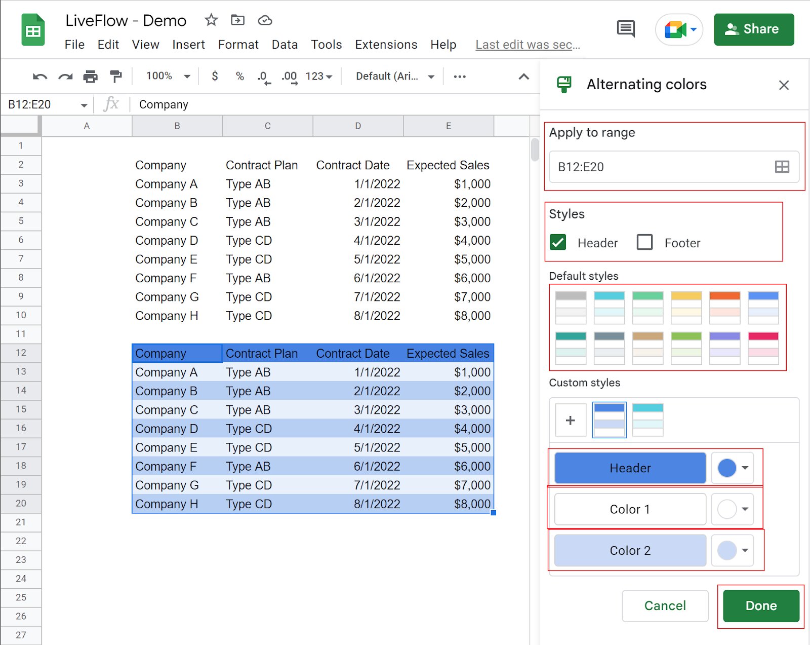
Step 4: Click on “Format” in the top menu and select “Alternating colors”

Now that you have selected the range of cells you want to apply alternating colors to, it’s time to access the formatting options in Google Sheets. You can easily access these options through the “Format” menu located at the top of the application.

Here’s how you can apply alternating colors to your selected range:

1. Click on the “Format” option in the top menu bar. This will open a drop-down menu with various formatting options.
2. From the drop-down menu, navigate to the “Alternating colors” option and click on it.

Upon selecting “Alternating colors,” a formatting sidebar will appear on the right side of the screen, providing you with additional customization options for the alternating color scheme.

By choosing the “Alternating colors” option, Google Sheets will automatically apply a default color scheme to the selected range. This default scheme typically consists of light and dark shades of the same color.

These alternating colors will make the rows or columns in your selected range visually distinct, allowing you to easily differentiate between different data points or entries. The alternating colors enhance the readability of your spreadsheet and facilitate data analysis.

Now that you have applied the default alternating colors scheme, feel free to proceed to the next step if you are satisfied with the default colors. However, if you wish to customize the color scheme, adjust the color options, or modify any other formatting attributes, continue reading to learn about the additional customization options available in Google Sheets.

Step 5: Choose the color scheme you want to use

After selecting the “Alternating colors” option in the format menu, you have the flexibility to choose the color scheme that best suits your preferences or matches the visual theme of your spreadsheet. Google Sheets provides a range of color options to choose from, allowing you to customize the appearance of your alternating colors.

To choose the color scheme you want to use, follow these steps:

1. In the formatting sidebar on the right side of the screen, you will see a section titled “Alternating colors”. This section provides various customization options for the color scheme.
2. Under the “Color scheme” option, click on the drop-down menu.
3. A list of predefined color schemes will appear. You can scroll through the options and choose the one that appeals to you.
4. As you select different color schemes, you can preview how they will look on your selected range in the spreadsheet.

Take your time to experiment with different color schemes until you find the one that enhances the readability and aesthetics of your data. Remember, the goal is to make the alternating colors visually pleasing and easy to distinguish.

Once you have chosen your preferred color scheme, proceed to the next step to further customize the color options if desired. However, if you are satisfied with the default color scheme and do not wish to make any further changes, you can skip the next step and move on to applying the selected color scheme.

Step 6: Adjust the color options if desired

Google Sheets offers additional customization options for the alternating colors scheme, allowing you to adjust the color options to better suit your preferences or specific requirements. These options enable you to fine-tune the colors used for the alternating rows or columns, providing you with more control over the appearance of your spreadsheet.

To adjust the color options, follow these steps:

1. In the formatting sidebar, locate the “Alternating colors” section.
2. Under the “Color options” subsection, you will find options to customize the colors for the even and odd rows or columns.
3. Click on the color box next to the respective option to open the color picker.
4. Within the color picker, you can choose a color from the spectrum, enter a specific color code, or use the sliders to adjust the RGB values.
5. As you make changes to the color options, the selected range will update in real-time, reflecting the modifications.

By adjusting the color options, you can create a more visually appealing and harmonious alternating colors scheme that aligns with your personal taste or project requirements. For example, you might opt for contrasting colors to make the alternating rows or columns stand out, or you may choose a more subtle color scheme for a calmer, less distracting appearance.

Feel free to experiment with different color combinations until you achieve the desired effect. You can always undo any changes or revert to the default color scheme if needed. Once you are satisfied with the color options, proceed to the next step to apply the alternating colors to your selected range.

Step 7: Click “Apply” to add alternating colors to your selected cells

After selecting the color scheme and making any desired adjustments to the color options, you are now ready to apply the alternating colors to your selected range of cells in Google Sheets. This step will finalize the formatting and add the chosen colors to the rows or columns you have specified.

To add the alternating colors to your selected cells, follow these simple steps:

1. In the formatting sidebar, review your chosen color scheme and color options to ensure they match your preferences.
2. Once you are satisfied with the settings, click on the “Apply” button located at the bottom of the formatting sidebar.

By clicking “Apply,” Google Sheets will immediately implement the alternating colors to the selected range. You will see the rows or columns in your range now displaying the chosen colors in the specified order.

Take a moment to review the applied alternating colors on your spreadsheet. Ensure that the colors are visually appealing, distinct, and aid in easy data interpretation. If any modifications are needed, you can go back and adjust the color scheme or options as desired.

Congratulations! You have successfully added alternating colors to your selected cells in Google Sheets. This formatting enhancement can greatly improve the readability and organization of your data, making it easier to identify patterns and analyze information.

Now that you have applied the alternating colors, it’s important to understand how to modify or remove them if needed. Let’s proceed to the next step to learn about making adjustments to the alternating colors in Google Sheets.

Step 8: Modify or remove alternating colors as needed

Once you have applied the alternating colors to your selected cells in Google Sheets, you may find the need to make modifications or even remove the alternating colors at some point. Luckily, Google Sheets provides easy-to-use options for adjusting and removing the applied formatting.

To modify or remove the alternating colors in your spreadsheet, follow these steps:

1. Ensure that the range with the alternating colors is still selected in your spreadsheet.
2. Click on the “Format” option in the top menu bar.
3. In the drop-down menu, select “Alternating colors” again.

By accessing the “Alternating colors” option once more, you will open the formatting sidebar that displays the current applied color scheme and options.

Here are the two methods you can use to make modifications or remove the alternating colors:

• Modifying: If you want to change the color scheme or color options, make the desired adjustments in the formatting sidebar. Once you are satisfied with the changes, click “Apply” to update the alternating colors.
• Removing: To remove the alternating colors completely, click on the “None” option in the color scheme drop-down menu. This will remove the applied formatting and revert the selected cells to their default appearance.

Using these options, you can modify the alternating colors whenever necessary or remove them entirely if they no longer serve your purpose. The flexibility to make modifications ensures that your spreadsheet’s appearance remains dynamic and adjustable to your needs.

With this final step, you have successfully learned how to modify or remove the alternating colors in Google Sheets. Feel free to experiment and make changes as needed to achieve the desired format for your spreadsheet.

Conclusion

Applying alternating colors to your data in Google Sheets can greatly improve the readability and organization of your spreadsheets. By visually separating rows or columns with different colors, you can easily identify patterns, compare data, and analyze information more effectively.

In this article, we walked through a step-by-step guide on how to make alternating colors in Google Sheets. We started by accessing Google Sheets and opening a new or existing spreadsheet. Then, we selected the range of cells we wanted to format and accessed the formatting options through the “Format” menu. Choosing a color scheme and adjusting the color options allowed us to customize the alternating colors according to our preferences.

Clicking “Apply” added the alternating colors scheme to our selected cells, enhancing the visual appeal of the spreadsheet. We also learned how to modify or remove the alternating colors in case any adjustments were needed down the line.

By applying these techniques, you can transform your spreadsheets into visually appealing and well-structured documents. Whether you’re organizing financial data, tracking project progress, or creating a simple list, the use of alternating colors can make your data stand out and make it easier to understand.

Now that you have mastered the process of making alternating colors in Google Sheets, feel free to get creative and experiment with different color schemes to find the perfect fit for your spreadsheets. With this powerful formatting feature at your disposal, you can create professional-looking spreadsheets that are both visually pleasing and easy to work with.

So go ahead, give it a try, and take your Google Sheets skills to the next level by adding alternating colors to your data!