How To Highlight A Row In Google Sheets

Introduction

Conditional formatting in Google Sheets allows you to apply specific formatting styles to cells based on certain conditions. It’s a powerful feature that can help you visually highlight important information and make your data more easily readable.

One of the useful applications of conditional formatting is to highlight an entire row based on the content of a specific cell. This can be particularly helpful when you want to emphasize certain data points or identify patterns in your data.

In this article, we will guide you through the process of highlighting a row in Google Sheets using conditional formatting. We will show you how to enable conditional formatting, select the range to be highlighted, choose the highlighting style, set the highlighting condition, apply the highlighting to the entire row, and how to remove the highlighting if needed.

By the end of this tutorial, you will have the knowledge and skills to effectively highlight rows in Google Sheets, empowering you to organize your data and present it in a visually appealing and easily understandable format.

Enable Conditional Formatting

Before you can start highlighting rows in Google Sheets, you need to enable the conditional formatting feature. Follow these steps to enable it:

1. Open your Google Sheets document.
2. Select the range of cells that you want to apply conditional formatting to. This can be a single cell, a range of cells, or the entire sheet.
3. Click on the “Format” tab in the menu bar at the top of the screen.
4. Select “Conditional formatting” from the dropdown menu.
5. A sidebar will appear on the right side of the screen. This is where you can configure your conditional formatting rules.
6. Choose the type of conditional formatting that you want to apply. You can choose from pre-defined rules or create custom rules based on formulas or cell values.
7. Specify the conditions under which the formatting should be applied. This can be based on text, numbers, dates, or custom formulas.
8. Customize the formatting style for the cells that meet the specified conditions. This can include changing the font color, background color, borders, and other formatting options.
9. Click on “Done” to apply the conditional formatting.

Once you have enabled conditional formatting, you can proceed to select the range to be highlighted and configure the highlighting style and conditions.

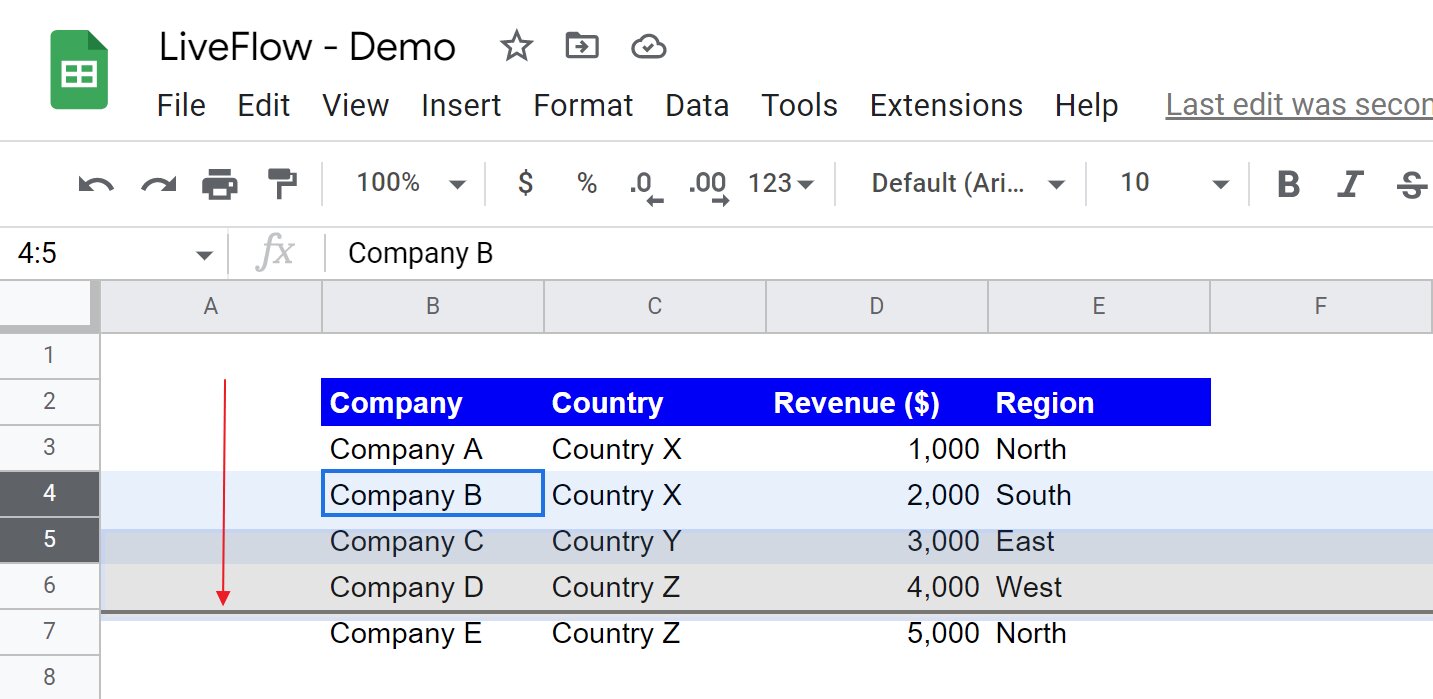
Select the Range to be Highlighted

After enabling conditional formatting in Google Sheets, the next step is to select the range of cells that you want to highlight as a row. Follow these steps to select the range:

1. Click on the first cell of the row that you want to highlight.
2. Drag your cursor across the row to select all the cells in that row.

If you want to highlight multiple rows, you can click and drag your cursor to select multiple rows in a similar manner.

Alternatively, if you want to highlight a specific range of cells that spans across multiple rows, you can click and drag your cursor to select the desired range.

Once you have selected the range of cells, you can proceed to choose the highlighting style and conditions for the conditional formatting.

Keep in mind that when applying the highlighting to an entire row, it’s important to select the entire row, including the cells with column labels or headers. This ensures that the highlighting is applied consistently to all the cells in the row.

Now that you have selected the range to be highlighted, let’s move on to the next step of choosing the highlighting style.

Choose the Highlighting Style

Once you have selected the range of cells to be highlighted in Google Sheets, the next step is to choose the highlighting style. This will determine how the highlighted row will visually appear in your spreadsheet.

To choose the highlighting style, follow these steps:

1. Click on the “Format” tab in the menu bar at the top of the screen.
2. Select “Conditional formatting” from the dropdown menu.
3. In the sidebar on the right, you will see the conditional formatting rules you previously set up. If you haven’t set up any rules yet, click on the “+” button to add a new rule.
4. Under the “Format cells if” section, you can specify the condition that triggers the highlighting. For example, you can highlight the row if a certain cell contains a specific value or meets a certain criteria.
5. Next, under the “Formatting style” section, click on the drop-down menu and choose the desired format for the highlighted row. This can include changing the font color, background color, borders, text style, or any other formatting option available.
6. You can also click on the “Add another rule” button to add multiple highlighting styles based on different conditions.
7. As you make changes to the highlighting style, you will see a preview of how the highlighted rows will appear in your spreadsheet.
8. Once you are satisfied with your highlighting style, click on “Done” to apply the changes.

By choosing the highlighting style, you can make the highlighted rows stand out in your spreadsheet, making it easier to identify important information or patterns in your data.

Now that you have chosen the highlighting style, let’s move on to setting the highlighting condition for the selected range.

Set the Highlighting Condition

After selecting the highlighting style for the rows in Google Sheets, the next step is to set the highlighting condition. This condition specifies when the highlighting should be applied to the selected range of cells.

To set the highlighting condition, follow these steps:

1. Click on the “Format” tab in the menu bar at the top of the screen.
2. Select “Conditional formatting” from the dropdown menu.
3. In the sidebar on the right, you will see the conditional formatting rules you previously set up. If you haven’t set up any rules yet, click on the “+” button to add a new rule.
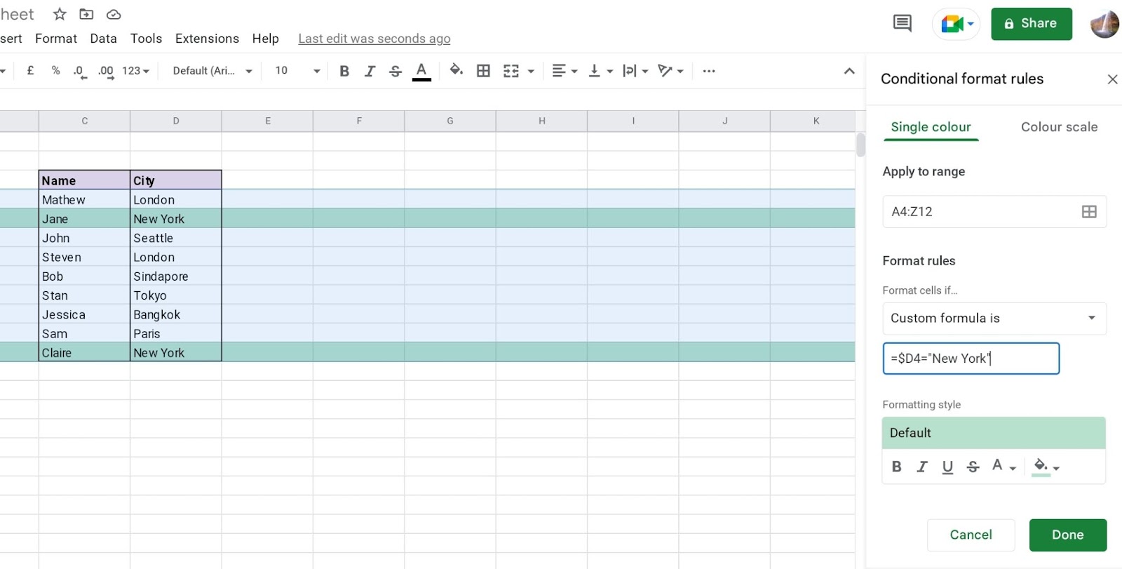
4. Under the “Format cells if” section, choose the condition that triggers the highlighting. This can be based on specific text, numerical comparisons, dates, or custom formulas.
5. Specify the condition by selecting the appropriate options such as “Text contains,” “Less than,” “Greater than,” “Is equal to,” or “Custom formula is.”
6. Enter the value or formula that determines the condition for highlighting. For example, if you want to highlight rows where a specific cell is equal to a certain value, enter that value in the provided field.
7. You can also add multiple conditions using the “Add another rule” button if you want to highlight rows based on different criteria.
8. As you set the highlighting condition, you can see a preview of how the highlighted rows will appear in your spreadsheet.
9. Once you have defined the highlighting condition, click on “Done” to apply the changes.

By setting the highlighting condition, you can specify the criteria that determine when the selected range of cells will be highlighted in Google Sheets.

Now that you have set the highlighting condition, let’s move on to applying the highlighting to the entire row.

Apply the Highlighting to the Entire Row

After setting the highlighting condition in Google Sheets, the next step is to apply the highlighting to the entire row. This ensures that the formatting is consistently applied to all the cells in the selected row based on the specified condition.

To apply the highlighting to the entire row, follow these steps:

1. Click on the “Format” tab in the menu bar at the top of the screen.
2. Select “Conditional formatting” from the dropdown menu.
3. In the sidebar on the right, you will see the conditional formatting rules you previously set up. If you haven’t set up any rules yet, click on the “+” button to add a new rule.
4. Under the “Range” section, make sure that the range of cells you want to apply the highlighting to is displayed correctly.
5. In the same section, select the option “Apply to range” and choose “Range” from the dropdown menu.
6. In the input box next to “Range,” specify the range of cells that covers the entire row you want to highlight. For example, if you selected the first cell of the row and dragged your cursor to cover the entire row, enter the range in the format “A1:X1” (where “X” corresponds to the last column in the row).
7. Make sure that the “Apply to” option is set to “Range” to ensure that the highlighting is applied to the entire row.
8. Click on “Done” to apply the changes and see the entire row highlighted based on the specified condition.

By applying the highlighting to the entire row, you ensure that the formatting is consistently applied to all the cells in the selected row, making it easier to identify and interpret the highlighted information.

Now that you have successfully applied the highlighting to the entire row, let’s explore how to remove the highlighting if needed.

Remove the Highlighting

If you no longer want to highlight a certain row or range of cells in Google Sheets, you can easily remove the highlighting. Here’s how:

1. Open your Google Sheets document.
2. Select the range of cells that have the highlighting that you want to remove. This can be a single cell, a range of cells, or the entire sheet.
3. Click on the “Format” tab in the menu bar at the top of the screen.
4. Select “Conditional formatting” from the dropdown menu.
5. A sidebar will appear on the right side of the screen. This is where you can manage your conditional formatting rules.
6. In the sidebar, you will see a list of the applied conditional formatting rules. Locate the rule that corresponds to the highlighting you want to remove.
7. Click on the trash bin icon next to the rule to delete it and remove the highlighting from the selected range of cells.
8. Click on “Done” to apply the changes and see the highlighting removed from the selected range of cells.

By removing the highlighting, you can revert the formatting of the cells back to their default appearance, allowing you to work with the data in its original state.

It’s important to note that removing the highlighting does not delete or modify the data in any way. It simply removes the visual formatting applied to the cells based on the conditional formatting rules.

With the knowledge of how to remove the highlighting, you can easily manage and update the conditional formatting in your Google Sheets document as needed.

Now that you know how to remove the highlighting, let’s summarize what we have covered in this tutorial.

Conclusion

Conditional formatting in Google Sheets is a valuable tool for highlighting specific rows based on certain conditions. By following the steps outlined in this tutorial, you can effectively highlight rows to draw attention to important data or recognize patterns in your spreadsheet.

We began by enabling conditional formatting and selecting the range of cells to be highlighted. We then moved on to choosing the highlighting style and setting the highlighting conditions based on specific criteria. Once the conditions were set, we applied the highlighting to the entire row, ensuring consistent formatting across all cells in the selected range.

If you ever want to remove the highlighting, we showed you how to easily delete the conditional formatting rule and revert the cells back to their original appearance.

By mastering the art of highlighting rows in Google Sheets, you can improve data analysis and presentation, making it easier for you and your audience to interpret and understand the information at a glance.

Remember, conditional formatting is a powerful feature that can be used in various scenarios, such as tracking expenses, monitoring sales, or organizing project data. Take advantage of this functionality to unlock the full potential of Google Sheets and optimize your workflow.

Now that you have the knowledge and skills to highlight rows in Google Sheets, it’s time to apply this technique to your own spreadsheets and make your data more visually appealing and informative.