How To Format Cell In Google Sheets

Introduction

Welcome to the world of Google Sheets formatting! If you’ve used Google Sheets before, you know that it’s a powerful tool for creating and organizing data. But did you know that you can also format your cells to make your spreadsheets more visually appealing and easier to understand?

Formatting cells in Google Sheets allows you to change the appearance of your data, such as the background color, font style, and alignment. Whether you’re working on a budget spreadsheet, a project tracker, or any other type of document, understanding how to format cells will help you present your data in a clear and professional way.

In this article, we will explore various formatting options in Google Sheets and learn how to make your spreadsheets look polished and organized. We’ll cover everything from changing the cell background color to applying conditional formatting and using custom formulas. By the end of this guide, you’ll have the skills to create visually stunning spreadsheets that make an impact.

Whether you’re a business professional, a student, or simply someone who needs to manage their personal finances, knowing how to format cells in Google Sheets will undoubtedly enhance your productivity and improve the overall appearance of your spreadsheets. So without further ado, let’s dive into the world of Google Sheets formatting and discover the endless possibilities!

Formatting Basics

Before we delve into the specific formatting options in Google Sheets, it’s important to understand the basics. Formatting cells in Google Sheets can be done through the toolbar at the top of the screen or by using keyboard shortcuts. Let’s take a look at some of the fundamental formatting techniques:

Highlighting Cells: To format a single cell or a range of cells, simply click and drag your cursor over the desired area. This will highlight the cells you want to format.
Toolbar Formatting: The toolbar at the top of the screen provides quick access to common formatting options. You can change the font style, font size, font color, and cell background color, among other things.
Keyboard Shortcuts: If you prefer using keyboard shortcuts to format cells, Google Sheets has you covered. For example, to make a cell bold, you can press Ctrl + B (or Command + B on Mac).

Now that we have a basic understanding of how formatting works in Google Sheets, let’s explore some of the specific formatting options available to us. From changing cell background color to applying number formats, we’ll cover a range of techniques to help you create professional and visually appealing spreadsheets.

Remember, the way you format your cells can greatly impact the readability and overall appeal of your spreadsheets. By using formatting techniques effectively, you can make your data easier to understand and navigate. So, let’s jump right into the world of Google Sheets formatting and unlock the full potential of your spreadsheets!

Changing Cell Background Color

One of the easiest ways to enhance the visual appeal of your Google Sheet is by changing the cell background color. This simple yet effective formatting option can help you organize your data, highlight important information, or create a visually cohesive design. Here’s how you can change the cell background color:

Select the cell or cells you want to change the background color for. You can click and drag your cursor to select multiple cells or use Shift + Click to select a range of cells.
In the toolbar at the top of the screen, click on the “Fill color” icon, represented by a paint bucket. This will open a color palette with various color options to choose from.
Click on the color you want to apply to your selected cells. The background color of the cells will instantly change to the selected color.

This feature is particularly useful when you want to visually differentiate specific cells or highlight important data. For example, you can use a different background color to indicate sales figures or to highlight important dates in a calendar.

Remember to use background colors strategically to maintain readability and contrast. Using colors that are too bright or too dark can make it difficult to read the data. It’s also a good idea to stick to a consistent color scheme throughout your spreadsheet to create a visually cohesive design.

By changing the cell background color in Google Sheets, you can transform your data into a visually appealing and well-organized spreadsheet. So, go ahead and experiment with different colors to make your data pop and grab the attention it deserves!

Changing Font Color

In addition to changing the background color of your cells, you can also customize the font color in Google Sheets. This allows you to emphasize certain data or make it stand out against the background color. Here’s how you can change the font color:

Select the cell or cells where you want to change the font color. You can select a single cell or click and drag your cursor to select multiple cells.
In the toolbar at the top of the screen, locate the “Font color” icon, represented by a letter “A” with a colored underline. Click on it to open the color palette.
Choose the desired font color by clicking on the color of your choice in the palette. The font color of the selected cells will change accordingly.

Changing the font color is a powerful formatting option that can help you draw attention to specific data or create a cohesive design by matching the font color with the overall color scheme of your spreadsheet. It’s important to consider the contrast between the font color and the background color to ensure readability.

For example, if you have a cell with a dark background color, using a light-colored font will improve readability. Similarly, if you have a light background color, using a darker font color will make the text easier to read.

Experimenting with different font colors can help you create emphasis, hierarchy, or visual interest in your spreadsheet. Whether you’re highlighting important values, categorizing data, or adding a personal touch to your document, changing the font color can make a big impact.

So go ahead and make your data stand out by customizing the font color in Google Sheets. By using this formatting option effectively, you can create visually appealing and well-organized spreadsheets that are both informative and visually engaging.

Applying Borders

In Google Sheets, applying borders to your cells can help you create clear divisions, highlight specific sections, or add a professional touch to your spreadsheet. Borders can be applied to individual cells, a range of cells, or the entire spreadsheet. Let’s explore how to apply borders in Google Sheets:

Select the cell or cells to which you want to apply borders. You can click and drag your cursor to select multiple cells or use Shift + Click to select a range of cells.
In the toolbar at the top of the screen, locate the “Borders” icon, represented by a grid pattern. Click on the icon to open the border options.
Choose the desired border style by clicking on the available options, such as solid, dashed, or dotted lines. You can also choose the border color and adjust the border thickness.

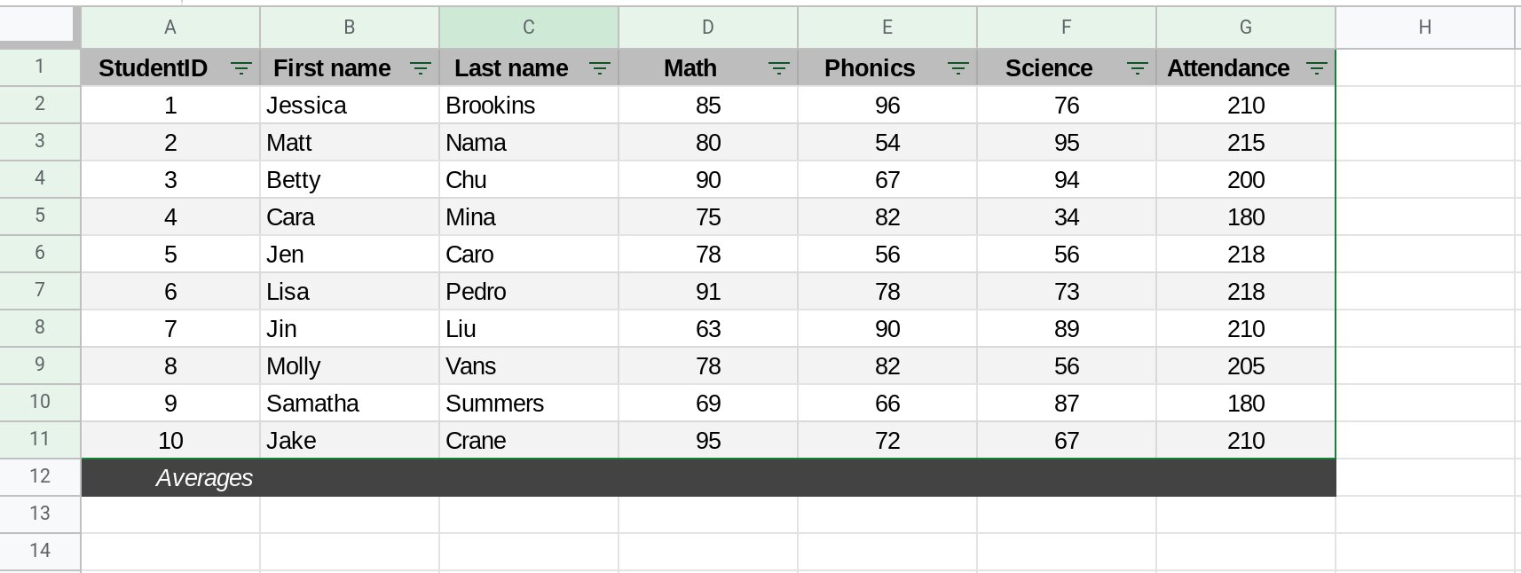
By applying borders to your cells, you can create clear visual separations between sections or highlight specific data points. For example, you might apply borders to create a table with distinct rows and columns, or use borders to enclose important figures or summaries.

Borders can also be used creatively to add a professional touch to your spreadsheet design. For instance, you might frame a title or header with a border to make it stand out, or use a double line border to highlight a subtotal or total.

Remember to use borders sparingly and strategically. Applying too many borders can clutter the spreadsheet and make it visually overwhelming. It’s important to strike a balance between adding structure and maintaining readability.

By applying borders to your cells in Google Sheets, you can add clarity, organization, and a touch of professionalism to your spreadsheets. So go ahead and experiment with different border styles and colors to create visually appealing and well-structured documents.

Applying Number Formats

In Google Sheets, applying number formats allows you to control how numerical data is displayed in your spreadsheet. Whether you’re working with currency, percentages, or dates, the number format feature gives you the flexibility to present your data in a way that is clear and meaningful. Here’s how you can apply number formats in Google Sheets:

Select the cell or cells that contain the numerical data you want to format. You can click and drag your cursor to select multiple cells or use Shift + Click to select a range of cells.
In the toolbar at the top of the screen, locate the “Number format” dropdown menu, represented by a set of numbers. Click on the dropdown menu to reveal the formatting options.
Choose the desired number format by selecting from the available options, such as “Currency”, “Percentage”, or “Date”. Depending on the format you choose, you may have additional options to customize the display of your data.

By applying number formats, you can enhance the readability and understandability of your data. For example, if you’re working with financial data, you might choose the currency format to display monetary values with currency symbols and decimal places. If you’re working with percentages, you can format the numbers accordingly to show them with a percentage symbol and the appropriate number of decimal places.

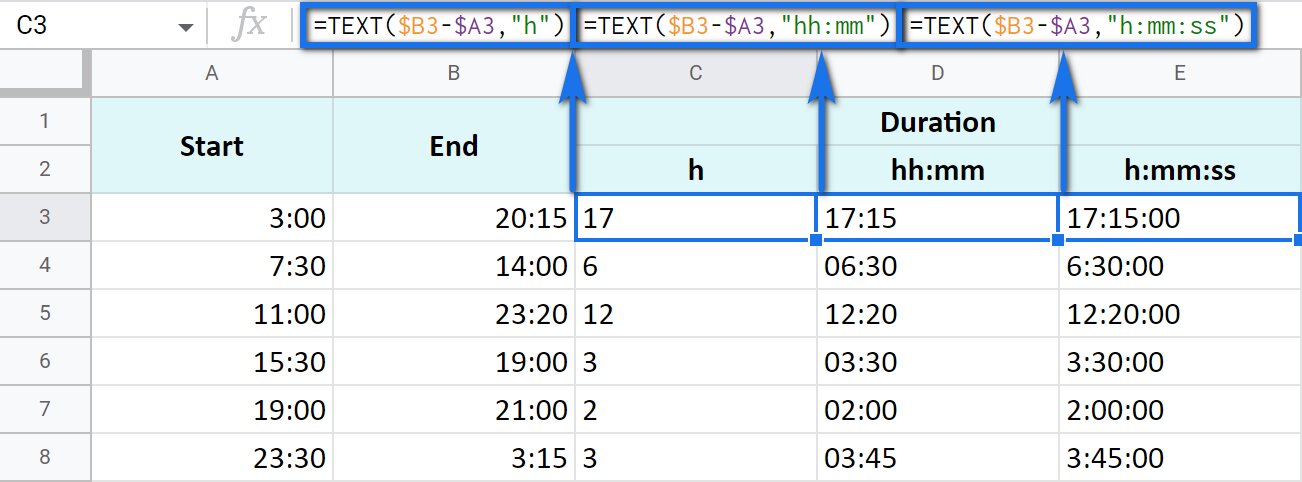
In addition to standard number formats, Google Sheets also allows you to create custom number formats. This gives you even more control over how your data is displayed. For example, you can create a custom number format to display negative numbers in red or apply specific formatting to different types of data within the same column.

Applying number formats not only improves the visual presentation of your spreadsheet but also helps to avoid misinterpretation of data. It ensures consistency in how numbers are formatted and makes it easier for others to understand and work with your data.

So, take advantage of the number format feature in Google Sheets and unleash the full potential of your numerical data. Whether it’s currency, percentages, or dates, the ability to format numbers allows you to effectively communicate your data in a clear and meaningful way.

Applying Conditional Formatting

In Google Sheets, conditional formatting is a powerful feature that allows you to automatically format cells based on specific criteria. With conditional formatting, you can visually highlight data that meets certain conditions, making it easier to identify trends, patterns, or outliers in your spreadsheet. Here’s how you can apply conditional formatting in Google Sheets:

Select the cell or cells that you want to apply conditional formatting to. You can click and drag your cursor to select multiple cells or use Shift + Click to select a range of cells.
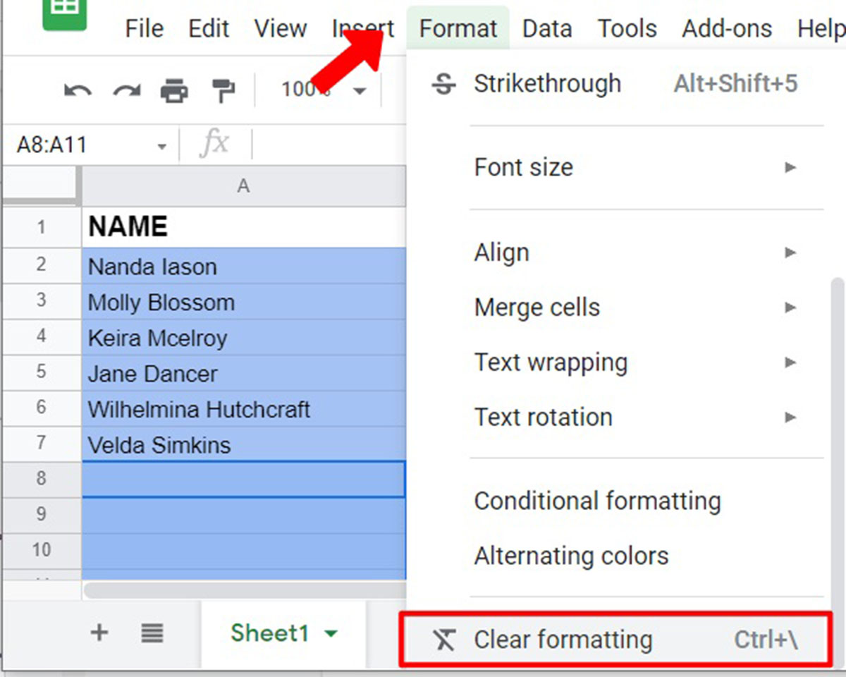
In the toolbar at the top of the screen, locate the “Format” dropdown menu. Click on the menu and select “Conditional formatting”.
A sidebar will appear on the right side of the screen, allowing you to set the conditions for formatting. Choose the criteria, such as greater than, less than, equal to, or between, and specify the value or range for the condition.
Select the formatting style you want to apply to the cells that meet the specified condition. This can include changing the font color, background color, or adding icons or data bars.
Click “Done” to apply the conditional formatting to the selected cells. The formatting will be automatically applied based on the conditions you set.

Conditional formatting is an incredibly useful tool for data analysis. It allows you to highlight specific data points that meet certain criteria without manually going through your entire spreadsheet. For example, you can use conditional formatting to identify the highest or lowest values in a range, highlight cells that contain specific text, or apply a color scale to visually represent the magnitude of values.

Furthermore, conditional formatting in Google Sheets is not limited to single-cell conditions. You can also apply conditional formatting rules that reference other cells or use custom formulas for complex conditions. This flexibility allows you to create dynamic and customized formatting based on your specific needs.

By applying conditional formatting, you can quickly identify important insights in your data and make informed decisions. It eliminates the need for manual data analysis and provides visual cues that draw attention to significant data points. Utilize this feature to efficiently analyze and present your data in a clear and meaningful way.

Merging Cells

In Google Sheets, merging cells allows you to combine multiple cells into a single, larger cell. This feature is particularly useful when you want to create headings, titles, or a more visually appealing layout in your spreadsheet. Here’s how you can merge cells in Google Sheets:

Select the cells that you want to merge. You can click and drag your cursor to select multiple cells or use Shift + Click to select a range of cells.
In the toolbar at the top of the screen, locate the “Merge cells” icon, represented by a set of merged cells. Click on the icon to merge the selected cells.
The selected cells will be merged into one larger cell. The content from the upper-left cell will be preserved, and the remaining cells will be combined into the merged cell, resulting in a single, larger cell.

Merging cells can help you create clear headings, labels, or titles for your data. For instance, if you have a table with multiple columns, you might want to merge the cells in the top row to create a header row that spans across all the columns. This makes it easier to identify the purpose of each column in your table.

It’s important to note that when you merge cells, the resulting merged cell inherits the formatting from the original upper-left cell. This includes the font style, font size, font color, and cell background color. So, if you want to change the formatting of the merged cell, you can do so by applying formatting directly to the merged cell.

However, it’s worth mentioning that while merging cells can be visually appealing, it can also impact the functionality of your spreadsheet. Merged cells cannot be sorted, filtered, or referenced in formulas. Therefore, it’s important to use merging cells appropriately and consider the potential impact on data manipulation and analysis.

Utilize the merging cell feature in Google Sheets to enhance the structure and readability of your spreadsheet. Whether it’s creating headers, labels, or a more aesthetically pleasing layout, merging cells can help you achieve a professional and organized look for your data.

Wrapping Text

In Google Sheets, wrapping text allows you to control how text is displayed within a cell. By default, long text strings are truncated, meaning that only a portion of the text is visible in the cell. However, by enabling text wrapping, you can make the entire text visible within the cell, improving readability and eliminating the need for manual resizing. Here’s how you can wrap text in Google Sheets:

Select the cell or cells in which you want to wrap the text. You can click and drag your cursor to select multiple cells or use Shift + Click to select a range of cells.
In the toolbar at the top of the screen, locate the “Wrap text” icon, represented by a diagonal arrow inside a box. Click on the icon to enable text wrapping for the selected cells.
The text within the selected cells will now be wrapped within the cell boundaries, making it fully visible. The row height will adjust automatically to accommodate the wrapped text.

Enabling text wrapping is particularly useful when you have lengthy text strings or when you want to display multiline text within a single cell. Whether it’s paragraph descriptions, comments, or labels, wrapping text ensures that all the text is visible without the need to resize columns or rows.

It’s important to note that when you wrap text in a cell, the row height is adjusted to fit the wrapped text. However, if the text in a cell exceeds the height of the row, you may need to manually adjust the row height to fully display the wrapped text. You can do this by dragging the row border or by using the “Resize row” option in the toolbar.

Text wrapping can also be combined with other formatting options, such as adjusting the font size or applying cell borders, to further enhance the visual presentation of your data.

By enabling text wrapping in Google Sheets, you can ensure that your text is fully visible within cells, improving readability and eliminating the need for manual adjustments. Utilize this feature to accommodate longer text strings, multiline descriptions, or any other content that requires visibility within cells.

Aligning Text

In Google Sheets, aligning text allows you to control the horizontal and vertical positioning of the text within a cell. This formatting option is essential for ensuring that your data is presented in a clear and organized manner. Whether you want to align text to the left, center, or right, or adjust the vertical alignment, Google Sheets provides several alignment options to meet your needs. Here’s how you can align text in Google Sheets:

Select the cell or cells that you want to align. You can click and drag your cursor to select multiple cells or use Shift + Click to select a range of cells.
In the toolbar at the top of the screen, locate the text alignment icons. These icons include left-align, center-align, right-align for horizontal alignment, and top-align, middle-align, bottom-align for vertical alignment.
Click on the desired alignment icon to apply the alignment to the selected cells. The text within the cells will adjust its position based on your chosen alignment settings.

Text alignment is crucial for presenting your data in a structured and visually appealing manner. By using appropriate text alignment, you can improve readability, create hierarchy, or emphasize important information.

For example, you might left-align text in a cell for labels or descriptions, center-align text for headers or titles, or right-align text for numerical data or currency values. Vertical alignment, on the other hand, allows you to control the positioning of the text within the cell, such as aligning it to the top, middle, or bottom.

Furthermore, you can combine different text alignment settings for cells within the same row or column to create visually dynamic layouts. This can be particularly useful for creating tables or organizing information in a comprehensive manner.

By using text alignment in Google Sheets, you can ensure that your data is presented in a neat and organized way. It helps to maintain consistency, readability, and clarity, resulting in a professional and visually appealing spreadsheet.

So go ahead and experiment with different text alignment settings to find the optimal arrangement for your data. Utilize the alignment options to create visually pleasing and structured spreadsheets that effectively communicate your information.

Changing Font Style

In Google Sheets, changing the font style allows you to modify the appearance of text within your spreadsheet. By selecting different font styles, you can add emphasis, create hierarchies, or enhance the overall aesthetic appeal of your data. Here’s how you can change the font style in Google Sheets:

Select the cell or cells that contain the text you want to modify. You can click and drag your cursor to select multiple cells or use Shift + Click to select a range of cells.
In the toolbar at the top of the screen, locate the “Font style” dropdown menu. Click on the menu and select from the available font styles. Google Sheets provides a variety of font styles, including bold, italic, and underline.
The selected text will immediately apply the chosen font style. You can also combine different font styles by applying multiple formatting options to the same cell or range of cells.

Changing the font style is a simple yet effective way to add visual impact to your spreadsheet. For example, using bold font can be useful for headers or important information that needs to stand out. Italicizing text can be helpful for emphasizing certain words or phrases, while underlining can be used for specific annotations or links.

In addition to the basic font styles, Google Sheets also allows you to customize the appearance of text further by adjusting the font color, size, and other formatting options. These additional settings give you more control over how your text is displayed and can help you create a cohesive visual design.

When choosing font styles, it’s essential to use them sparingly and consistently throughout your spreadsheet. Too many font styles can create visual clutter and make your data harder to read. It’s best to use different font styles purposefully, highlighting only the most important information or using them to create a hierarchy within your data.

By changing the font style in Google Sheets, you can make your text more visually appealing, improve readability, and highlight essential elements. So, feel free to experiment with different font styles and create a text appearance that suits the purpose and aesthetics of your spreadsheet.

Changing Font Size

In Google Sheets, changing the font size allows you to adjust the size of the text displayed within your spreadsheet. By modifying the font size, you can improve readability, draw attention to specific information, or create a visually balanced layout. Here’s how you can change the font size in Google Sheets:

Select the cell or cells containing the text you want to modify. You can click and drag your cursor to select multiple cells or use Shift + Click to select a range of cells.
In the toolbar at the top of the screen, locate the “Font size” dropdown menu. Click on the menu and select from the available font sizes. Google Sheets provides a range of font sizes, from small to large.
The selected text will immediately adjust to the chosen font size. You can also apply different font sizes to various cells to create a diverse and visually engaging design.

Changing the font size is an effective way to enhance the readability and visual appeal of your spreadsheet. Larger font sizes are often used for headers or titles, allowing them to stand out and be easily noticed. On the other hand, smaller font sizes can be useful for less prominent information or when you need to fit more text within a cell.

It’s important to strike a balance when choosing font sizes. Using an overly large font size can lead to clutter and an unprofessional appearance, while using a very small font size may compromise readability, especially for smaller screens or when printing the spreadsheet.

In addition to adjusting the font size of individual cells, Google Sheets also allows you to apply formatting to entire columns, rows, or even the entire spreadsheet. This can be helpful when you want consistency in the font size across multiple cells or when you want to quickly change the font size of a large portion of your data.

By changing the font size in Google Sheets, you can customize the appearance of your text to suit your needs. Whether it’s creating headers, emphasizing key information, or optimizing readability, font size plays a crucial role in effectively presenting your data.

So go ahead and experiment with different font sizes to find the optimal balance for your spreadsheet. Make sure the text is easily readable and visually appealing, and consider the overall design and purpose of your document as you make your font size selections.

Adding Cell Notes

Google Sheets allows you to add cell notes, which are small text-based annotations that provide additional information or context about specific cells. These notes can be helpful for documenting important details, clarifying formulas, or providing instructions to other collaborators. Here’s how you can add cell notes in Google Sheets:

Right-click on the cell where you want to add a note, and select “Insert note” from the context menu. Alternatively, you can go to the “Insert” menu at the top of the screen, hover over “Note,” and select “Insert note” from the dropdown menu.
A small rectangular box will appear within the cell, indicating the note. Click inside the box to type your note.
Save the note by pressing Enter or clicking outside the note box. The note will now be linked to the cell and displayed as a small red triangle in the upper-right corner of the cell.

Cell notes are a valuable tool for providing additional information without cluttering the main spreadsheet. They can be especially useful when working with complex formulas, datasets, or when collaborating with others. Cell notes remain hidden until you hover over the linked cell, making it easy to view and access essential information when needed.

In addition to adding text-based notes, you can also format the text within the note using basic formatting options such as bold, italic, and underline. This allows you to highlight specific details or differentiate important information within the note itself.

Collaborators with access to the spreadsheet can view and reply to the cell notes, making them a great tool for communication and collaboration. To view or reply to a note, simply hover over the linked cell, click on the red triangle, and a small pop-up will appear, displaying the note and any existing replies.

By utilizing cell notes in Google Sheets, you can enhance the clarity and documentation of your spreadsheet. These notes serve as a helpful reference, guiding both yourself and others through the data and contributing to better organization and understanding of the information at hand.

So, add cell notes to your Google Sheets whenever you need to provide additional context or instructions. Use them to make your spreadsheet more informative and actionable, ensuring that important information is readily available to all those who access your document.

Applying Text Rotation

In Google Sheets, text rotation allows you to change the orientation of text within cells. This feature is particularly useful when you want to fit more content into a narrow column, create headers or labels that span multiple rows, or simply add visual interest to your spreadsheet. Here’s how you can apply text rotation in Google Sheets:

Select the cell or cells that contain the text you want to rotate. You can click and drag your cursor to select multiple cells or use Shift + Click to select a range of cells.
In the toolbar at the top of the screen, locate the “Text rotation” icon. It is represented by a square with an angled arrow. Click on the icon to open a dropdown menu of rotation options.
Choose the desired text rotation option from the available presets, such as rotating the text to a specific angle or changing the orientation to vertical or diagonal.

Applying text rotation can help you maximize the use of limited space in your spreadsheet and make your data more organized and visually appealing. By rotating text, you can fit longer headers or labels into narrower columns, improving readability and conserving space.

In addition to the preset rotation options, you can also set custom text rotation angles to meet your specific formatting needs. This flexibility allows you to create unique visual effects or align the text in a way that best suits the purpose of your spreadsheet.

Text rotation is especially useful when you want to create multicolumn headers, such as when building a table or chart. By rotating text and spanning it across multiple rows, you can clearly define the relationship between columns and provide descriptive labels for each data category.

It’s important to note that when you apply text rotation, the row height or column width may need to be adjusted to accommodate the rotated text properly. Auto-adjusting row height and column width can be done manually by dragging the boundary lines or using the “Resize row” or “Resize column” options in the toolbar.

Use text rotation creatively to add visual interest and improve the readability of your spreadsheet. It’s a simple yet effective way to optimize space, highlight headers or labels, and organize your data in a visually appealing manner.

By applying text rotation in Google Sheets, you can create a unique and engaging presentation of your data. Explore the different rotation options and don’t be afraid to experiment and find the text orientation that best suits your specific formatting needs.

Using Data Validation

In Google Sheets, data validation is a powerful feature that allows you to control the type and range of data that can be entered into a cell. By setting up data validation rules, you can ensure data accuracy, prevent errors, and maintain consistency in your spreadsheet. Here’s how you can use data validation in Google Sheets:

Select the cell or cells where you want to apply data validation. You can click and drag your cursor to select multiple cells or use Shift + Click to select a range of cells.
In the toolbar at the top of the screen, go to the “Data” menu and select “Data validation.”
A dialog box will appear with various options for setting up data validation. You can choose from a range of validation criteria, such as whole numbers, dates, text length, or even create custom formulas.
Specify the validation criteria and any additional settings, such as error messages or custom help text, to guide users entering data into the cells.
Click “Save” to apply the data validation rules to the selected cells.

Data validation is particularly useful when you want to maintain data integrity and ensure that only valid and consistent data is entered into cells. It can be applied to a variety of scenarios, such as restricting input to specific date ranges, allowing only numerical values within a certain range, or validating text entries based on length or specific patterns.

When data validation is applied to a cell, any user attempting to enter data that doesn’t meet the validation criteria will be alerted with an error message. This helps to prevent incorrect or inconsistent data from being entered, thus improving the quality and reliability of your spreadsheet.

Moreover, data validation can also include custom help text, which provides additional instructions or explanations to users regarding the data entry requirements. This can be especially useful when collaborating with others or sharing the spreadsheet with individuals who may not be familiar with the specific data requirements.

By utilizing data validation in Google Sheets, you can effectively manage and control the data entered into your spreadsheet. This feature ensures data accuracy and consistency, saves time by reducing user errors, and increases the overall reliability and usability of your spreadsheet.

So, take advantage of data validation to enforce data integrity and improve the quality of your spreadsheet. Set up validation rules that suit your specific data requirements and ensure that your data remains reliable and consistent throughout your Google Sheets document.

Using Custom Formulas for Conditional Formatting

In Google Sheets, custom formulas for conditional formatting allow you to apply formatting rules based on complex logical expressions. While the built-in conditional formatting options cover many scenarios, custom formulas provide the flexibility to create advanced formatting rules that are specific to your needs. Here’s how you can use custom formulas for conditional formatting:

Select the cell or cells that you want to apply conditional formatting to. You can click and drag your cursor to select multiple cells or use Shift + Click to select a range of cells.
In the toolbar at the top of the screen, go to the “Format” menu and select “Conditional formatting.”
In the sidebar that appears on the right side of the screen, select “Custom formula” as the formatting rule.
Enter your custom formula in the input field provided. The formula should evaluate to either TRUE or FALSE for each cell in the selected range.
Specify the desired formatting options, such as font color, background color, or border style, for cells that meet the condition.
Click “Done” to apply the custom formula to the selected cells. The formatting will be automatically applied based on the evaluation of the formula.

Using custom formulas for conditional formatting allows you to create sophisticated rules based on your specific requirements. You can combine different criteria, reference other cells or ranges, and utilize various logical operators and functions to define the formatting conditions.

For example, you can create a custom formula to highlight cells that contain specific text, flag values that meet certain numerical conditions, or format cells based on more intricate logical expressions. Custom formulas provide the flexibility to apply conditional formatting based on the unique characteristics of your data and the insights you want to extract.

Additionally, custom formulas for conditional formatting can be particularly helpful for data analysis and visualization. By applying custom formatting rules, you can draw attention to important trends, identify outliers, or visualize patterns that are not covered by the built-in formatting options.

Make sure to test and validate your custom formulas to ensure they produce the desired formatting results. You can verify the outcome by modifying the data in the selected cells or evaluating the formula on a smaller sample range before applying it to the entire dataset.

By utilizing custom formulas for conditional formatting in Google Sheets, you can unlock a world of possibilities for visually enhancing your data. Experiment with different formulas, explore the available functions and operators, and use custom formatting to uncover valuable insights and present your data in a visually impactful way.

Using Cell Styles

In Google Sheets, cell styles provide a quick and efficient way to apply consistent formatting to your spreadsheet. With a variety of pre-defined cell styles available, you can instantly give your data a professional and polished look. Here’s how you can use cell styles in Google Sheets:

Select the cell or cells that you want to format with a cell style. You can click and drag your cursor to select multiple cells or use Shift + Click to select a range of cells.
In the toolbar at the top of the screen, go to the “Format” menu and select “Cell styles.”
A drop-down menu will appear, displaying a range of cell style options. Hover over each style to see a live preview of how it will appear in your selected cells.
Click on the desired cell style to apply it to the selected cells. The formatting will be instantly applied, including changes to font size, font color, background color, borders, and other style elements.

Cell styles are designed to save you time and effort by providing a consistent and professional formatting option. They offer a range of styles, from headers and titles to data rows and footers. Whether you’re creating a financial report, a project plan, or a simple table, cell styles can significantly enhance the visual presentation of your data.

Besides the built-in cell styles, you can also create your own custom cell styles. Custom cell styles allow you to define specific formatting rules and apply them to cells throughout your spreadsheet. This feature is particularly handy when you have a unique formatting requirement that is not covered by the default cell styles.

As you apply cell styles, you have the flexibility to modify or override individual formatting elements within the selected cells. For example, you can adjust the font size, change the font color, or customize the cell background color to further align with your specific needs.

By utilizing cell styles in Google Sheets, you can achieve consistency and professionalism throughout your spreadsheet. This feature not only saves time on repetitive formatting tasks but also ensures that your data is presented in a visually appealing and cohesive manner.

So, explore the various cell styles available in Google Sheets and find the one that best suits your needs. Experiment with custom cell styles to create a unique formatting style for your specific spreadsheet requirements. Cell styles are a powerful tool for elevating the visual impact of your data and making your spreadsheet look organized and visually impressive.

Using Keyboard Shortcuts

In Google Sheets, keyboard shortcuts are a time-saving feature that allow you to quickly perform various actions without the need to navigate through menus or use the mouse. By memorizing and utilizing keyboard shortcuts, you can improve your efficiency and productivity while working with spreadsheets. Here’s how you can use keyboard shortcuts in Google Sheets:

Navigation:

Arrow keys: Use the arrow keys to navigate to adjacent cells in the direction of the arrow.
Tab: Move one cell to the right.
Shift + Tab: Move one cell to the left.
Enter: Move one cell down.
Shift + Enter: Move one cell up.
Ctrl + Home: Jump to the top-left cell of the sheet.
Ctrl + End: Jump to the bottom-right cell of the sheet.

Formatting:

Ctrl + B: Apply or remove bold formatting to selected text.
Ctrl + I: Apply or remove italic formatting to selected text.
Ctrl + U: Apply or remove underline formatting to selected text.
Ctrl + Shift + F: Open the format options for selected cells.
Ctrl + Shift + L: Apply or remove a bullet list formatting to selected cells.
Ctrl + Shift + C: Copy formatting from selected cells.
Ctrl + Shift + V: Paste formatting to selected cells.

Data and Formulas:

Ctrl + C: Copy selected cells.
Ctrl + X: Cut selected cells.
Ctrl + V: Paste copied or cut cells.
Ctrl + Z: Undo the last action.
Ctrl + Y: Redo the last undone action.
Ctrl + D: Fill down the selected cell with the contents of the top cell in the column.
Ctrl + ; (semicolon): Insert the current date in the selected cell.
Ctrl + Shift + ; (semicolon): Insert the current time in the selected cell.

Using keyboard shortcuts can significantly enhance your efficiency and speed while working in Google Sheets. By memorizing these shortcuts and incorporating them into your workflow, you can streamline your spreadsheet tasks and reduce reliance on the mouse or touchpad.

It’s worth noting that keyboard shortcuts may vary slightly based on your operating system and browser. Additionally, you can access the full list of available shortcuts by pressing Ctrl + / (forward slash) or Cmd + / (forward slash) on a Mac. This will open a dialog box with the complete list of keyboard shortcuts for Google Sheets.

So, familiarize yourself with the commonly used keyboard shortcuts and gradually incorporate them into your workflow. With practice, you’ll become more efficient and proficient in navigating and formatting your spreadsheets, ultimately saving time and improving your overall productivity.