How To Make Table In Google Sheets

Introduction

Welcome to the world of Google Sheets! Whether you’re a seasoned number-cruncher or just starting to dive into the world of spreadsheets, Google Sheets is a powerful tool that can help you organize data, create reports, and collaborate with others. In this article, we’ll guide you through the process of creating and formatting tables in Google Sheets.

Tables are essential for organizing and displaying data in a structured manner. Google Sheets provides a user-friendly interface that allows you to effortlessly create tables and customize them to suit your needs. With its cloud-based nature, you can access and edit your tables anywhere, anytime, and easily collaborate with others in real-time.

Whether you’re tracking sales data, managing inventory, or analyzing survey results, Google Sheets’ table features will make your life easier. In this guide, we will cover the fundamental aspects of creating and formatting tables in Google Sheets, as well as utilizing advanced functionalities such as sorting, filtering, and using formulas.

Before we dive in, it’s worth mentioning that basic familiarity with Google Sheets’ interface and functions will be helpful. If you’re new to Google Sheets, don’t worry! We’ll provide step-by-step instructions to ensure you’re on the right track.

So, let’s get started on our journey to become Google Sheets table maestros. By the end of this article, you’ll be equipped with the knowledge and skills to create visually appealing and efficient tables that will elevate your data management tasks to a whole new level.

Getting started with Google Sheets

Before we jump into creating tables, let’s familiarize ourselves with Google Sheets. If you’re new to Google Sheets or need a refresher, this section will provide you with the basics to navigate and utilize this powerful spreadsheet software.

Google Sheets is a web-based application that allows you to create, edit, and collaborate on spreadsheets online. It is available for free to anyone with a Google account, making it accessible to individuals and businesses alike. To get started, simply go to Google Sheets (sheets.google.com) and sign in with your Google account credentials.

Once you’re logged in, you’ll be greeted with a blank spreadsheet, also known as a sheet. Google Sheets utilizes a grid system consisting of columns labeled with letters (A, B, C, etc.) and rows labeled with numbers (1, 2, 3, etc.). This grid layout allows you to organize data into cells and manipulate them as needed.

At the top of the screen, you’ll find the toolbar, which houses various menus and buttons for formatting, inserting data, and performing other actions. The toolbar can be customized to suit your preferences, allowing you to have quick access to the features you use most frequently.

One of the remarkable features of Google Sheets is its ability to collaborate in real-time. You can share your spreadsheet with others by clicking on the “Share” button in the top-right corner. By entering the email addresses of your collaborators, you can grant them view or edit access to the sheet. This makes Google Sheets an excellent tool for team projects or sharing information with clients or colleagues.

Google Sheets offers a wide range of functions and formulas to perform calculations and automate processes. These functions can be accessed through the “Functions” button on the toolbar or by manually typing them into the desired cell. From simple addition and subtraction to more complex statistical analyses, Google Sheets has you covered.

Now that you have a basic understanding of Google Sheets’ interface and functionalities, we can move on to creating our tables. In the next section, we’ll walk through the process of creating a new sheet and entering data into it. So, let’s roll up our sleeves and get ready to excel!

Creating a new sheet

Creating a new sheet in Google Sheets is a breeze. Whether you want to start fresh or organize your data into separate sheets, here’s a step-by-step guide on how to create a new sheet:

1. Open Google Sheets and sign in to your account.
2. On the main toolbar, click on the “+” icon or go to “File” and select “New Spreadsheet.”
3. A new blank sheet will open in a new tab. If you prefer to have multiple sheets within the same spreadsheet, you can click on the “+” icon at the bottom of the screen to add more sheets.
4. To rename the sheet, simply double-click on the default name, “Sheet1,” and enter a new name that reflects the purpose of the sheet. For example, if you’re creating a table to track expenses, you can name it “Expense Tracker.”

That’s it! You’ve successfully created a new sheet in Google Sheets. Now it’s time to enter data and start building your table.

It’s important to note that Google Sheets allows you to have multiple sheets within the same spreadsheet. This can be incredibly useful when you want to organize your data into different categories or when working on complex projects that require multiple sheets for different purposes.

To navigate between sheets, you can simply click on the sheet’s tab at the bottom of the screen. Each sheet has its own unique name and can be customized further with different formatting options to distinguish them from one another.

Creating multiple sheets within the same spreadsheet enables you to reference data from one sheet to another, making data analysis and manipulation more efficient. This feature is particularly helpful when working with large datasets or when you need to consolidate information from different sources.

In the next section, we’ll dive into entering data into the sheet and explore various formatting options to make your table visually appealing and easy to read. So, let’s move on to the next step in our journey towards mastering Google Sheets!

Entering data into the sheet

Now that you have created a new sheet in Google Sheets, it’s time to start populating it with data. Whether you’re working with numerical values, text, or a combination of both, Google Sheets provides a user-friendly interface for entering and managing your data. Here’s how to enter data into the sheet:

1. Select the cell where you want to enter your data. You can do this by clicking on the desired cell on the grid.
2. Type in the data you wish to enter. It can be numbers, text, dates, or other types of information.
3. Press Enter on your keyboard to move to the next cell below or use the arrow keys to navigate to a different cell.

You can also copy and paste data from other sources, such as a spreadsheet or a text document, into Google Sheets. Simply select the data you want to copy, right-click, and choose the “Copy” option. Then, navigate to your Google Sheets, select the cell where you want to paste the data, right-click, and choose the “Paste” option.

If you have a large dataset, you may find it more efficient to use the drag-to-fill feature in Google Sheets. This allows you to quickly fill a series or pattern of data into adjacent cells. To use this feature, enter the initial value in a cell, and then click and drag the fill handle (the small square in the bottom-right corner of the selected cell) across the range of cells you want to fill. Google Sheets will automatically populate the cells with the appropriate values based on the pattern you set.

In addition to entering data into individual cells, you can also merge cells to create a larger field for entering text or formatting purposes. To merge cells, select the range of cells you want to merge, right-click, and choose the “Merge cells” option from the dropdown menu.

Once you have entered your data into the sheet, you can further customize the appearance of the cells by adjusting the font, font size, font color, cell borders, and more. These formatting options can be accessed through the toolbar at the top of the screen or by right-clicking on the selected cells and choosing the desired formatting option.

Now that you know how to enter and format your data, it’s time to take it a step further and format your sheet as a table. In the next section, we’ll explore how to insert a table in Google Sheets and make it visually appealing. So, let’s continue our journey towards becoming Google Sheets experts!

Formatting the sheet

Formatting your sheet in Google Sheets allows you to enhance the visual appeal and readability of your data. It enables you to highlight important information, apply consistent styles, and make your table more visually engaging. Here are some ways to format your sheet:

Cell formatting: To format individual cells, select the desired cells and use the toolbar options or right-click menu to change the font, font size, font color, background color, and alignment. You can also apply different number formats, such as currency or percentage, to numeric data.

Conditional formatting: Conditional formatting is a powerful feature in Google Sheets that allows you to automatically apply formatting based on specific conditions. For example, you can highlight cells that meet certain criteria, such as values above or below a threshold, by choosing from a variety of formatting styles. This makes it easier to visually analyze your data and identify patterns or outliers.

Applying cell borders: To create a clear separation between cells or groups of cells, you can add borders. Select the cells you want to apply the border to, click on the “Borders” button in the toolbar, and choose the desired border style and thickness.

Formatting as a table: Google Sheets allows you to format your data as a table, which applies a consistent style to the entire range of data. To do this, select the range of cells you want to format, click on the “Format” menu, go to “Table,” and choose the desired table style. Formatting as a table not only improves the visual organization of your data but also enables you to sort and filter your table easily.

Freezing rows and columns: If you have a large table with many rows or columns, it can be helpful to freeze certain rows or columns so that they stay visible while you scroll through the rest of the sheet. To do this, select the row or column you want to freeze, click on the “View” menu, go to “Freeze,” and choose the appropriate option.

Applying themes: To quickly apply a pre-designed style to your entire sheet, you can use themes. Click on the “Format” menu, go to “Theme,” and choose the desired theme. This will change the font, colors, and formatting of your entire sheet, giving it a cohesive and professional look.

Remember that formatting is not just about making your sheet visually appealing. It also plays a crucial role in improving readability, emphasizing important information, and creating a consistent and professional look. Experiment with different formatting options to find the style that best suits your needs and enhances the presentation of your data.

In the next section, we’ll explore how to insert a table into your Google Sheets and adjust its size and position. So, let’s continue our journey towards mastering Google Sheets!

Inserting a table

Now that you have entered and formatted your data, it’s time to organize it into a table format. Google Sheets makes it easy to insert a table and customize it to fit your needs. Here’s how to insert a table in Google Sheets:

1. Select the range of cells that you want to include in your table. This can be a single row or column, or a larger range that contains multiple rows and columns.
2. With the selected cells highlighted, click on the “Insert” menu at the top of the screen and choose the “Table” option. Alternatively, you can right-click on the selected cells and select “Table” from the dropdown menu.
3. A dialog box will appear, allowing you to customize the appearance of your table. You can choose whether the table has headers, select a table style, and adjust other formatting options.
4. Click on the “Insert” button to insert the table into your sheet. The selected cells will now be organized into a visually appealing table with headers, if applicable.

Once inserted, you can easily modify your table by adding or removing rows and columns, adjusting the size and position, and applying further formatting options.

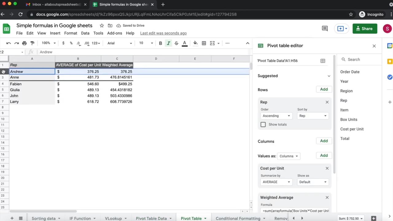
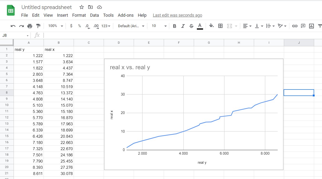
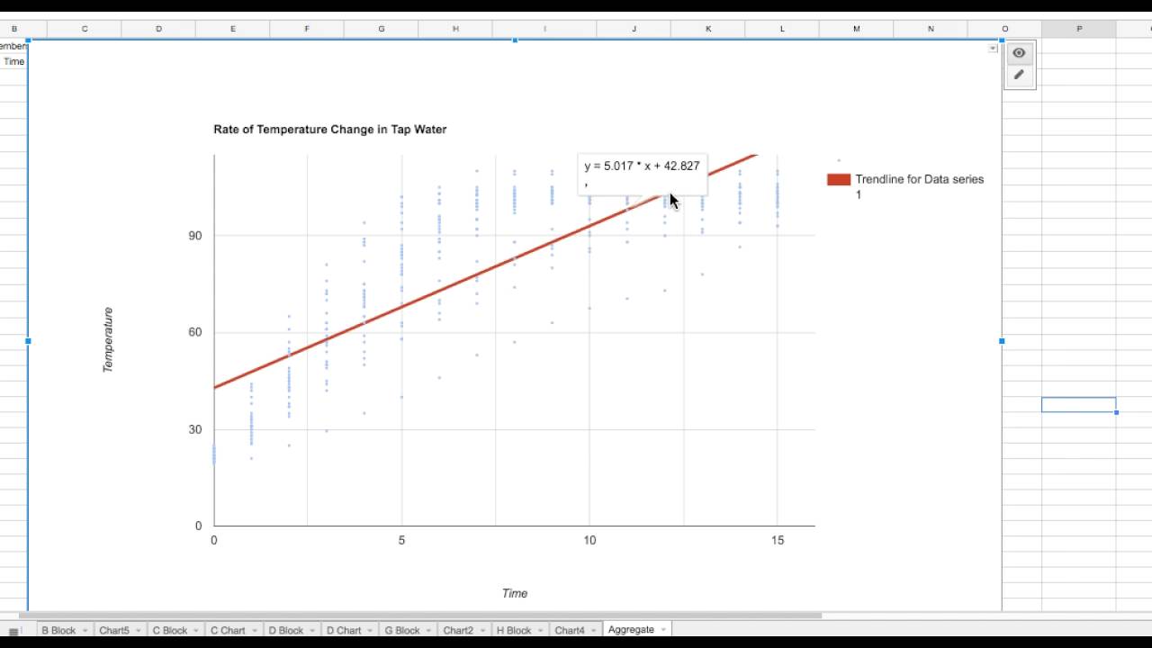
Google Sheets also provides a useful feature called “Explore” that allows you to generate charts and analyze data within your table. To access Explore, click on the “Explore” button located at the bottom-right corner of the screen. Explore will provide you with insights and suggestions to gain deeper insights into your data.

As tables are dynamic, any changes you make to the underlying data will automatically update the table. This makes Google Sheets a powerful tool for managing and analyzing data in real-time. You can even link your table to other sheets or external data sources to ensure that your table reflects the most up-to-date information.

Now that you have successfully inserted a table into your Google Sheets, it’s time to learn how to adjust its size and position within the sheet. In the next section, we’ll explore these customization options, so let’s continue our journey towards becoming Google Sheets experts!

Adjusting the table size and position

After inserting a table in Google Sheets, you may find the need to adjust its size and position to better fit your layout and make it visually appealing. Google Sheets provides various options to customize the size and position of your table. Here’s how to adjust the table size and position:

Resizing the table: To resize your table, click on any corner of the table and drag it to expand or shrink it. You can adjust the width and height of the table as needed to accommodate your data or fit it within a specific space on your sheet.

Adding or removing rows and columns: To add a row or column to your table, right-click on the table and choose the “Insert” option from the dropdown menu. You can then select whether you want to insert a row above or below the selected row, or a column to the left or right of the selected column. To remove a row or column, right-click on the corresponding row or column and choose the “Delete” option.

Moving the table: You can move the table to a different location on your sheet by clicking and dragging the table from the top-left corner. This allows you to reposition the table and adjust its alignment with other elements on the sheet.

Merging and splitting cells: You can merge cells within your table to create larger fields or to format specific sections. To merge cells, select the cells you want to merge, right-click, and choose the “Merge cells” option. To split merged cells back into individual cells, select the merged cells, right-click, and choose the “Split cells” option.

Aligning the table: To align the table within the sheet, select the table and use the toolbar options to adjust the horizontal and vertical alignment. This helps in achieving a consistent layout and ensures that the table fits seamlessly with the rest of your content.

By customizing the size and position of your table, you can effectively present your data and make it more visually appealing. Take advantage of these features to create a well-organized and visually appealing sheet that showcases your data effectively.

Now that you know how to adjust the size and position of your table, let’s move on to the next section where we will explore how to add and remove rows and columns within the table. So, let’s continue our journey towards mastering Google Sheets!

Adding and removing rows and columns

Google Sheets allows you to easily add or remove rows and columns within your table. This flexibility enables you to adjust the structure of your table as your data changes or when you need to insert new information. Here’s how to add and remove rows and columns in Google Sheets:

Adding rows:

1. Select the row below which you want to add a new row.
2. Right-click on the selected row and choose the “Insert 1 above” option if you want to add a single row or “Insert 10 above” to add multiple rows at once.

Adding columns:

1. Select the column to the right of which you want to add a new column.
2. Right-click on the selected column and choose the “Insert 1 left” option if you want to add a single column or “Insert 10 left” to add multiple columns at once.

Google Sheets will insert the new rows or columns, pushing the existing data down or to the right, while preserving the formatting of your table.

Removing rows:

1. Select the row or rows that you want to remove.
2. Right-click on the selected row(s) and choose the “Delete row” option. Alternatively, you can use the “Delete” key on your keyboard.

Removing columns:

1. Select the column or columns that you want to remove.
2. Right-click on the selected column(s) and choose the “Delete column” option. Alternatively, you can use the “Delete” key on your keyboard.

Removing rows or columns will delete the selected data and shift the remaining data up or to the left, ensuring that your table remains contiguous and well-structured.

These techniques allow you to easily adjust the size and structure of your table, ensuring that it remains aligned with your data and meets your evolving needs. Whether you need to insert new rows or columns, or remove unnecessary ones, Google Sheets provides the flexibility to keep your table organized and optimized.

In the next section, we’ll explore how to format your table to make it more visually appealing and easy to navigate. So, let’s continue our journey towards becoming Google Sheets experts!

Formatting the table

Formatting your table in Google Sheets can greatly enhance its visual clarity and make it easier to read and understand. With various formatting options available, you can customize the appearance of your table to suit your specific needs. Here’s how to format your table in Google Sheets:

Applying table styles: Google Sheets offers a range of predefined table styles that you can apply to your table with just a few clicks. To apply a table style, select the table and click on the “Format” menu. From there, go to “Table” and choose the table style that best suits your aesthetic preferences or complements the overall design of your sheet. Applying a table style will instantly update the appearance of your entire table, including headers, borders, and alternating row colors, providing a consistent and visually pleasing look.

Adjusting cell formatting: To further customize the appearance of your table, you can format individual cells or groups of cells by modifying font styles, sizes, colors, and alignments. You can also add conditional formatting to highlight specific data based on certain criteria. For example, you can apply different background colors to cells based on their values or set up data bars to visually represent the magnitude of values within a range. By utilizing cell formatting and conditional formatting, you can emphasize important information and make your table easier to interpret at a glance.

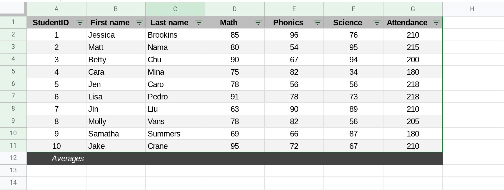
Adding headers and totals: Headers and totals help to provide context and summary information within a table. You can designate a header row to label the columns in your table, making it easier to identify and understand the data. Similarly, you can add a footer row to display summary totals or calculations for each column. To add headers or totals, simply select the row where you want to add them and apply the desired formatting.

Adjusting column widths: Google Sheets allows you to manually adjust the width of individual columns to accommodate different data types and ensure optimal readability. To adjust column width, hover your cursor over the boundary line between two column headers until it changes into a double-sided arrow. Then, click and drag the boundary line left or right to increase or decrease the column width according to your preference.

Freezing rows or columns: If your table has a large number of rows or columns, you may want to freeze certain rows or columns so that they remain visible while scrolling through the rest of the table. Freezing rows or columns can be especially useful when you have headers or totals that you want to keep in view. Simply select the row or column below or to the right of the desired frozen section, go to the “View” menu, and choose “Freeze” to freeze the necessary rows or columns.

Merging and splitting cells: To combine cells within your table, enabling you to have larger fields for text or formatting purposes, select the cells you want to merge and use the “Merge cells” option from the right-click menu or the toolbar. Conversely, if you need to split previously merged cells back into individual cells, select the merged cells and choose the “Split cells” option. This flexibility allows you to arrange your data and format it in a way that best suits your presentation needs.

By utilizing these formatting options, you can transform your table into a visually appealing and organized representation of your data. Formatting plays a vital role in making your table more digestible and conveying information effectively to your audience.

In the next section, we’ll explore how to sort and filter the data in your Google Sheets table, providing you with powerful tools for data analysis. So, let’s continue our journey to becoming Google Sheets experts!

Sorting and filtering table data

Sorting and filtering are essential tools in Google Sheets that allow you to analyze and manipulate data within your table. With these features, you can easily find specific information, identify trends, and make sense of complex datasets. Here’s how to sort and filter data in your Google Sheets table:

Sorting data:

1. Select the entire range of your table, including headers, that you want to sort.
2. Click on the “Data” menu and choose the “Sort range” option.
3. In the dialog box that appears, select the column you want to sort by from the “Sort by” dropdown menu.
4. Choose whether you want to sort in ascending or descending order.
5. Click on the “Sort” button to apply the sorting to your table.

Google Sheets will rearrange your data based on the selected column, placing the values in the chosen order. Sorting your data allows you to easily organize it in ascending or descending order and quickly identify the highest or lowest values, alphabetical listings, or other patterns within your table.

Filtering data:

1. Select the entire range of your table, including headers, that you want to filter.
2. Click on the “Data” menu and choose the “Create a filter” option.
3. Arrows will appear in each header cell. Click on the arrow in the column by which you want to filter your data.
4. A dropdown menu will appear, allowing you to select specific criteria for filtering.
5. Choose the desired filtering options, such as equal to, greater than, contains, or custom formulas.
6. Click on the “OK” button to apply the filter to your table.

By filtering your data, you can temporarily hide rows that do not meet your specified criteria. This allows you to focus on specific subsets of data and perform more targeted analysis. Additionally, you can combine multiple filters to further refine your results and gain deeper insights into your data.

Both sorting and filtering are dynamic features, meaning that if your data changes or if you update your table, you can reapply sorting and filtering options to reflect the latest information. This flexibility ensures that your analysis remains up to date and accurate.

Now that you know how to sort and filter your table data, you can easily organize and analyze your information. In the next section, we’ll explore how to use formulas within your table cells to perform calculations and automate processes. So, let’s continue our journey to becoming Google Sheets experts!

Using formulas in the table cells

Formulas are a powerful feature in Google Sheets that allow you to perform calculations, manipulate data, and automate processes within your table. By utilizing formulas, you can save time, minimize errors, and extract valuable insights from your data. Here’s how to use formulas in the cells of your Google Sheets table:

Entering a formula:

1. Select the cell where you want the result of your formula to appear.
2. Start the formula with an equals sign (=) followed by the desired formula expression.
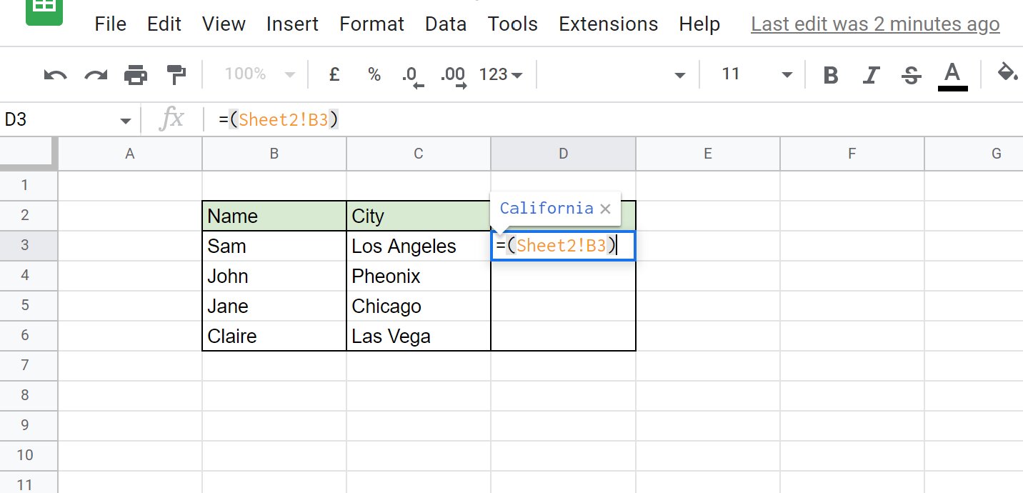
3. Refer to other cells in your table by their cell references. For example, to add the values in cells A1 and A2, use the formula =A1+A2.
4. Use parentheses to specify the order of operations if needed. For example, to multiply the sum of cells A1 and A2 by the value in cell B1, use the formula =(A1+A2)*B1.
5. Press Enter on your keyboard to calculate the result of the formula and display it in the cell.

Commonly used formulas:

Google Sheets offers a wide range of predefined functions that you can use in your formulas. Some commonly used functions include:

• SUM: Calculates the sum of a range of cells. For example, =SUM(A1:A5) adds the values in cells A1 to A5.
• AVERAGE: Calculates the average of a range of cells. For example, =AVERAGE(B1:B10) calculates the average of the values in cells B1 to B10.
• MAX: Returns the maximum value from a range of cells. For example, =MAX(C1:C20) returns the highest value in cells C1 to C20.
• MIN: Returns the minimum value from a range of cells. For example, =MIN(D1:D15) returns the lowest value in cells D1 to D15.
• COUNT: Counts the number of cells in a range that contain numerical values. For example, =COUNT(E1:E30) counts the cells in cells E1 to E30 that have numerical values.

These are just a few examples of the countless functions available in Google Sheets. You can explore the full range of functions by clicking on the “Functions” button in the toolbar or by using the “Insert function” option in the right-click menu.

Formulas in Google Sheets are dynamic, meaning that if the underlying data in your table changes, the formula will automatically recalculate and update the result. This ensures the accuracy and efficiency of your calculations, even as your data evolves.

Using formulas allows you to unlock the full potential of your data in Google Sheets. By performing calculations, aggregating data, and automating processes, you can gain valuable insights and streamline your workflow.

In the next section, we’ll explore how to collaborate on your Google Sheets table, making it easier to work with others and share your data securely. So, let’s continue our journey to becoming Google Sheets experts!

Collaborating on the table

One of the most powerful features of Google Sheets is its ability to collaborate with others in real-time. Whether you’re working on a team project, sharing data with colleagues, or gathering feedback from clients, Google Sheets provides seamless collaboration tools that make working together a breeze. Here’s how to collaborate on your Google Sheets table:

Sharing the table:

1. Click on the “Share” button located in the top-right corner of the screen.
2. Enter the email addresses of the people you want to collaborate with, choosing whether to grant them view-only or edit access.
3. Customize the access permissions by clicking on the drop-down menu next to each person’s email address. You can allow them to view, comment, or edit the sheet, depending on their role and the level of access you want to grant.
4. Click on the “Send” button to share the table with the specified people.

Once shared, each collaborator will be able to access the table through their own Google account. They can view and interact with the data in real-time, allowing for seamless collaboration and instant updates.

Collaboration features:

Google Sheets provides a variety of collaboration features to enhance teamwork and streamline communication:

• Comments: Collaborators can leave comments on specific cells or ranges within the table, creating a discussion thread for feedback, suggestions, or questions. To add a comment, simply right-click on a cell and select “Insert comment.”
• Chat: The built-in chat function allows collaborators to communicate with each other within the Google Sheets interface. Click on the chat icon on the right side of the screen to open the chat panel and start a conversation with your collaborators.
• Revision history: Google Sheets keeps a detailed revision history that tracks changes made to the table. You can access the revision history by clicking on “File” in the toolbar and selecting “Version history.” This feature allows you to go back to previous versions, compare changes, and restore earlier versions if needed.
• Real-time updates: All changes are reflected in real-time, so collaborators can instantly see the updates made by others. This ensures that everyone is working on the most up-to-date version of the table and prevents version control issues.
• Collaborator presence: Google Sheets shows you who else is currently viewing or editing the table, represented by colored cursor indicators. This provides visibility into who is actively working on the table at any given time.

Collaborating on a Google Sheets table enables multiple users to work together, share ideas, and contribute to the data analysis process. Whether you’re refining calculations, making data-driven decisions, or simply gathering input from various stakeholders, collaborating in real-time enhances productivity and ensures a more efficient workflow.

Now that you know how to collaborate on your Google Sheets table, you can harness the power of teamwork and make the most out of your shared data. In the next section, we’ll wrap up our journey on Google Sheets and recap what we’ve learned. So, let’s conclude our exploration of Google Sheets!

Conclusion

Congratulations! You have now gained valuable insights into how to create, format, and collaborate on tables in Google Sheets. From understanding the basics of Google Sheets to inserting and formatting tables, you have learned the fundamental skills needed to manage and analyze your data effectively.

You discovered how to create new sheets and enter data into them, along with formatting options to improve the visual appeal of your tables. By adjusting the size and position of tables, merging cells, and applying conditional formatting, you can enhance the clarity and organization of your data.

You also explored powerful features such as sorting and filtering, enabling you to quickly analyze and find specific information within your tables. You learned how to use formulas to perform calculations and automate processes, allowing you to unlock the full potential of your data.

Furthermore, you discovered the importance of collaboration in Google Sheets. By sharing your tables and utilizing the commenting and chat features, you can foster teamwork, gather feedback, and make real-time updates with your collaborators.

Google Sheets empowers you to become a master of your data and streamline your workflow. Whether you’re an individual managing personal finances, a team working on a project, or a business analyzing sales data, Google Sheets provides the tools you need to make informed decisions and drive success.

Remember, practice is key to mastering these skills. Continue exploring Google Sheets, experimenting with different features, and finding creative ways to visualize and analyze your data. In no time, you’ll become an expert in creating and managing powerful tables in Google Sheets.

So, go ahead, embrace the world of Google Sheets, and take full advantage of its capabilities to streamline your data management and analysis. Have fun and happy spreadsheeting!