Choosing the Right Template
When it comes to working with Google Sheets, starting with the right template can make a significant difference in your productivity. Google Sheets offers a wide range of templates that are tailored to various needs and industries, allowing you to jumpstart your project with ease and efficiency.
Before diving into the available templates, it’s important to have a clear understanding of your goals and requirements. Whether you’re managing personal finances, organizing a team project, or tracking sales data, there is likely a template that suits your needs.
To begin, open Google Sheets and click on the “Template Gallery” option. This will take you to a library of pre-designed templates across different categories. You can browse through the options or use the search bar to find templates related to your specific task.
The template categories cover a wide array of purposes, such as budgeting, project management, calendars, inventory tracking, and more. Take your time to explore the templates that catch your interest and note down their names or bookmark them for later access.
Once you have selected a template, click on “Use Template” to create a new spreadsheet based on your chosen design. The template will open in a new tab, ready for you to customize and input your data. Most templates come with predefined formulas and formatting, which can save you time and effort in setting up your spreadsheet from scratch.
It’s important to choose a template that aligns with your specific needs but also allows room for customization. While templates provide a solid foundation, you may need to tailor them to suit the unique requirements of your project or organization. Look for templates that offer flexibility and the ability to add or modify columns, rows, and formulas as necessary.
Remember, the right template is a powerful tool that can streamline your work and enhance productivity. Choosing the appropriate template from the start will save you valuable time, help you stay organized, and ensure that your spreadsheet meets your objectives.
Creating a New Spreadsheet
In Google Sheets, creating a new spreadsheet is a straightforward process that allows you to start organizing and analyzing your data. Whether you’re starting from scratch or using a template, here’s a step-by-step guide to help you get started:
- Open Google Sheets by visiting the Google Sheets website or accessing it through your Google Drive.
- Click on the “+ New” button located in the upper-left corner of the screen. A dropdown menu will appear.
- Select “Google Sheets” from the dropdown menu. This will open a blank spreadsheet in a new tab.
- At this point, you can begin customizing your spreadsheet by adding headers, labels, and data. Click on a cell and start typing to enter data.
- To add rows or columns, right-click on the row or column header and select “Insert” from the dropdown menu. A new row or column will be added above or to the left of the selected cell.
- To format the appearance of your spreadsheet, highlight the desired cells and use the toolbar options at the top of the page. You can change the font, color, alignment, and more.
- To save your work, click on the “File” tab in the top left corner and select “Save” or use the keyboard shortcut Ctrl + S (Windows) or Command + S (Mac).
- If you want to name your spreadsheet, click on the current title located at the top of the page, next to the Google Sheets logo. Enter a new name and press Enter.
- To share your spreadsheet with others, click on the blue “Share” button in the top-right corner. Enter the email addresses of the individuals you want to collaborate with and choose their level of access.
- Finally, if you prefer to work offline, you can enable the “Offline” mode by clicking on the “Settings” tab in the top-right corner and selecting “Offline.” This will allow you to access and edit your spreadsheet even without an internet connection.
Creating a new spreadsheet in Google Sheets is a simple yet powerful way to organize and analyze your data. By following these steps, you’ll be well on your way to creating a customized spreadsheet tailored to your unique needs.
Navigating the Google Sheets Interface
When working with Google Sheets, getting familiar with the interface and its various features is important for efficient navigation and usage. Here’s a guide on how to navigate the Google Sheets interface:
- Menu Bar: The menu bar is located at the top of the page and contains various options such as File, Edit, View, Insert, Format, and more. These options allow you to perform different actions and make changes to your spreadsheet.
- Toolbar: The toolbar is situated just below the menu bar and offers quick access to formatting options, including font style, font size, text alignment, cell background color, and more. It also includes buttons for common actions like Undo, Redo, and Save.
- Ribbon: The ribbon is a section below the toolbar that provides additional functionalities and options. It contains different tabs, such as Home, Insert, Format, Data, and more, each with its own set of related tools and features.
- Formula Bar: The formula bar is located below the ribbon and displays the contents of the currently selected cell. You can enter and edit formulas directly into the formula bar to perform calculations and manipulate data.
- Sheets Tab Bar: The sheets tab bar is at the bottom of the screen and shows the names of all the sheets in your spreadsheet. You can click on a sheet tab to switch between sheets and access their individual contents.
- Grid: The main area of the interface is the grid, which consists of rows and columns of cells. This is where you enter and manipulate your data. You can click on a cell to select it, and use the arrow keys to navigate through adjacent cells.
- Zoom Controls: In the bottom-right corner of the screen, you’ll find zoom controls that allow you to adjust the view of your spreadsheet. You can zoom in to see more details or zoom out to see a larger portion of your data.
- View options: Google Sheets offers various view options to help you customize your working environment. From the “View” tab in the menu bar, you can choose to show or hide gridlines, freeze rows or columns, adjust the zoom, and more.
- Collaboration Tools: Google Sheets is designed for collaboration, allowing multiple users to work on the same spreadsheet simultaneously. The interface displays the names or icons of collaborators who are currently editing the spreadsheet, and you can use the “Share” button to invite others to collaborate.
By familiarizing yourself with the different elements of the Google Sheets interface, you’ll be able to navigate through your spreadsheets with ease and make the most of the available tools and features.
Entering Data into Cells
Entering data into cells is the fundamental step in creating and populating your Google Sheets spreadsheet. Whether you’re inputting numerical values, text, or formulas, here are the essential techniques to enter data:
- Selecting a Cell: To begin, click on the cell where you want to enter your data. The selected cell will be highlighted to indicate that it is the active cell. You can navigate to different cells using the arrow keys on your keyboard.
- Typing Directly into Cells: The simplest way to enter data is by typing directly into the active cell. Click on the cell and start typing to input your text or numbers. Press Enter or use the arrow keys to move to the next cell.
- Auto-Filling Cells: Google Sheets has a powerful auto-fill feature that allows you to quickly populate a series of cells with a pattern. To use this feature, enter a value into a cell and then click and drag the small blue square located in the bottom-right corner of the cell to fill adjacent cells with the pattern.
- Pasting Data: If you have data saved elsewhere, you can easily paste it into your spreadsheet. First, copy the data from its original source. Then, click on the destination cell in your spreadsheet and choose “Paste” from the Edit menu or use the Ctrl + V (Windows) or Command + V (Mac) keyboard shortcut.
- Importing Data: If you have a large dataset or data in a different format, you can import it into Google Sheets. From the File menu, select “Import” and choose the appropriate option to import data from another spreadsheet, CSV file, or external source.
- Adding Formulas: Formulas are a powerful tool in Google Sheets that allow you to perform calculations and manipulate data. To add a formula, start by typing the equals sign “=” into the cell where you want the result to appear. Then, enter the formula using functions, cell references, and operators.
- Using Functions: Google Sheets offers a vast range of built-in functions that can help you analyze and manipulate your data. Functions such as SUM, AVERAGE, COUNT, and IF are commonly used in calculations. To use a function, start typing the function name followed by an opening parenthesis “(” and enter the necessary arguments or cell references.
- Editing Data: To change the data in a cell, double-click on the cell, or select the cell and press F2. This will activate edit mode, allowing you to modify the content of the cell. After making your changes, press Enter to save the edited data.
By mastering the skills of entering data into cells, you will be able to populate your Google Sheets spreadsheet accurately and efficiently. Whether it’s simple text, numerical values, or complex formulas, you’ll have the tools needed to organize and analyze your data effectively.
Formatting Cells and Data
Formatting cells and data in Google Sheets allows you to enhance the appearance, readability, and organization of your spreadsheet. Here are some key formatting options to help you make your data more visually appealing and easier to interpret:
- Changing Font Styles: To change the font style, size, and color of your text, use the formatting options on the toolbar or the Format menu. You can select a range of cells and apply formatting to the entire selection or choose specific cells to format individually.
- Applying Cell Borders: Borders can be used to visually separate and define different sections of your spreadsheet. To add borders, select the desired cells or range and use the formatting options to choose the border style and thickness.
- Adjusting Cell Alignment: Proper alignment can significantly improve the readability of your data. Use the alignment options in the toolbar to align text horizontally or vertically within cells, as well as to wrap text within a cell if necessary.
- Applying Number Formats: Number formatting helps you display values in a consistent and meaningful way. To format numerical data, select the cells or range, and use the Format menu or the toolbar options to choose from options like currency, decimal places, percentages, and more.
- Conditional Formatting: Conditional formatting enables you to highlight cells that meet specific criteria. With this feature, you can emphasize data trends, identify outliers, or draw attention to important values. Use the “Format” menu and select “Conditional formatting” to set up custom rules and formatting styles.
- Applying Cell Fill Colors: Cell fill colors can be used to visually group or categorize data. Select the cells or range and use the fill color options in the toolbar to apply different background colors. This can help you differentiate data or highlight specific information.
- Merging Cells: Merging cells allows you to combine multiple cells into a single larger cell. This can be useful for creating headers or labels that span across multiple columns or rows. Select the cells you want to merge, right-click, and choose the “Merge cells” option from the context menu.
- Applying Cell Formats: In addition to number formats, Google Sheets offers various other formatting options, such as date formats, text styles, special formats for URLs, and more. Use the Format menu or the formatting options on the toolbar to apply the desired format to your selected cells.
- Copying Formatting: If you have already formatted a cell or a range of cells and want to apply the same formatting to another area, you can use the “Format Painter” tool. Select the cell with the desired formatting, click on the paintbrush icon in the toolbar, and then select the cells you want to apply the formatting to.
By utilizing these formatting options, you can present your data in a visually appealing and organized manner, enhancing its readability and impact. Experiment with different formatting techniques to create clear and professional-looking spreadsheets that effectively communicate your data.
Adding Formulas and Functions
Formulas and functions are powerful tools in Google Sheets that enable you to perform calculations, manipulate data, and automate tasks within your spreadsheet. Here’s a guide on how to add formulas and functions to your Google Sheets:
- Entering Formulas: To add a formula, start by selecting the cell where you want the result to appear. Then, type the equals sign “=” to indicate that you are entering a formula. You can now enter the formula using mathematical operators (+, -, *, /), cell references, and functions. Google Sheets provides a wide range of built-in functions to perform various calculations and data manipulations.
- Using Functions: Functions are predefined formulas that perform specific calculations or operations. To use a function, start by typing the function name followed by an opening parenthesis “(” and enter the necessary arguments or cell references within the parentheses. Google Sheets offers a comprehensive library of functions, including mathematical, statistical, logical, text, date, and more. You can use the “Insert” menu or the Functions button on the toolbar to browse and select functions.
- Referencing Cells: When adding formulas or functions, referencing cells is crucial. You can reference a cell by simply typing its address, such as A1 or B2. For more complex formulas, you can also use relative references (e.g., A1, B1) to refer to cells relative to the active cell, or absolute references (e.g., $A$1, $B$1) to refer to specific cells that should not change when the formula is copied or dragged.
- Copying Formulas: Once you have entered a formula, you can easily apply it to other cells by copying or dragging the formula. Simply click on the cell with the formula, and then move your cursor to the small blue square in the bottom-right corner of the cell. Click and drag the square to copy the formula to adjacent cells. Google Sheets will adjust the cell references automatically to match the new locations.
- Error Checking: Google Sheets has built-in error checking features to help you identify and correct formula errors. If a formula returns an error, an alert triangle will appear in the cell. You can click on the triangle to see a brief explanation of the error and suggestions on how to fix it. Google Sheets also highlights error cells with a red border.
- Conditional Formulas: Conditional formulas allow you to perform calculations based on certain conditions. You can use logical functions like IF, AND, OR, and others to create formulas that generate different results depending on specified criteria. Conditional formulas are useful for data analysis, decision-making, and creating dynamic reports.
By utilizing formulas and functions in Google Sheets, you can automate calculations, manipulate data, and unlock greater insights within your spreadsheet. Experiment with different formulas and explore the extensive library of functions to unleash the full potential of your data analysis and processing capabilities.
Sorting and Filtering Data
In Google Sheets, sorting and filtering data allows you to quickly organize and analyze your spreadsheet based on specific criteria. Whether you’re working with a small dataset or a large collection of information, sorting and filtering can help you gain insights and make data-driven decisions. Here’s how to sort and filter data in Google Sheets:
- Sorting Data: To sort data, select the range of cells you want to sort. Then, click on the “Data” tab in the menu bar and choose either “Sort sheet by column” or “Sort range.” You can choose to sort in ascending or descending order by selecting the desired option. Additionally, you can sort by multiple columns to further refine the sorting criteria.
- Filtering Data: Filtering allows you to display only specific rows of data that meet certain criteria. To apply a filter, select the range you want to filter, and click on the “Data” tab in the menu bar. Choose the “Create a filter” option. Filter arrows will appear in the header row of each column. Click on the filter arrow of a column to display the filter options, and then select or deselect the criteria you want to filter by.
- Custom Filtering: Google Sheets provides a range of custom filter options for more advanced filtering. You can use filter conditions such as greater than, less than, equal to, contains text, and more. These options allow you to create specific criteria that match your data analysis needs. Select the range you want to filter, click on the filter arrow, and choose “Filter by condition” to access the custom filter options.
- Clearing Sorting and Filtering: To remove sorting or filtering from your data, you can click on the “Data” tab and select “Turn off sorting” or “Turn off filter.” This will revert the data to its original order and display all the rows.
- Sorting and Filtering Across Multiple Sheets: If you have multiple sheets in your spreadsheet and you want to sort or filter data across all sheets simultaneously, you can use the “Data” tab and select “Sort range” or “Filter” options. Ensure that all the relevant sheets are selected or included in the range before applying the sorting or filtering.
- Sorting and Filtering Options: Google Sheets offers various sorting and filtering options beyond simple alphabetical or numerical ordering. For example, you can sort by color, sort by date, or filter based on the values in a specific range. These options provide additional flexibility to customize the sorting and filtering process to suit your needs.
Sorting and filtering data in Google Sheets are essential techniques for managing and analyzing large sets of information. By organizing your data in a meaningful and structured way, you can quickly identify patterns, spot trends, and extract valuable insights from your spreadsheet.
Creating Charts and Graphs
In Google Sheets, creating charts and graphs is an effective way to visually represent your data and communicate insights in a more engaging and easy-to-understand format. Charts and graphs can help you identify patterns, trends, and relationships within your spreadsheet. Here’s how to create charts and graphs in Google Sheets:
- Selecting Data: Before creating a chart or graph, you need to select the data you want to include. Highlight the range of cells that contain the data you want to visualize. Include column headers if you want them to be included as labels in the chart.
- Inserting a Chart: With the data selected, go to the “Insert” menu and choose “Chart.” A sidebar will appear on the right-hand side of the screen with different chart types to choose from.
- Choosing a Chart Type: Google Sheets offers a variety of chart types, including column charts, line charts, pie charts, bar charts, scatter plots, and more. Explore the different options and select the chart type that best represents your data and suits your analysis goals.
- Customizing the Chart: Once you have selected a chart type, you can customize its appearance and layout. Use the options in the sidebar to modify the chart’s title, labels, axis titles, colors, fonts, and more. You can also choose to display or hide specific elements like gridlines or data points.
- Updating Chart Data: If you make changes to the data in your spreadsheet, Google Sheets will automatically update the chart to reflect those changes. You can also manually update the chart by selecting it and clicking on the chart editor button in the toolbar. This allows you to add or remove data series, modify the range of data, and adjust other chart settings.
- Moving and Resizing the Chart: Google Sheets allows you to move and resize the chart to better fit within your spreadsheet or presentation. Click and drag the chart to reposition it, and use the resizing handles to adjust its size. You can also place the chart on a separate sheet by selecting “Move to own sheet” from the chart editor.
- Embedding the Chart: If you want to share or publish the chart outside of Google Sheets, you can easily embed it in other platforms like websites or documents. Select the chart, click on the “Edit” tab in the chart editor, and choose the “Publish chart…” option. Follow the prompts to generate an embed code that you can insert into your desired platform.
Creating charts and graphs in Google Sheets helps you to visually explore and communicate patterns and trends in your data. Experiment with different chart types and customization options to find the best way to present your information and emphasize the insights you want to share.
Collaborating with Others
One of the key advantages of using Google Sheets is its ability to facilitate seamless collaboration with others. Whether it’s for team projects, data analysis, or financial planning, collaborating with others in real-time can greatly enhance productivity and efficiency. Here’s how to collaborate with others in Google Sheets:
- Sharing your Spreadsheet: To collaborate with others, you need to share your Google Sheets spreadsheet. Click on the blue “Share” button in the top-right corner of the screen. Enter the email addresses of the people you want to collaborate with, and choose their level of access – can view, can comment, or can edit. You can also generate a shareable link to distribute to others.
- Real-time Editing: Google Sheets allows multiple users to edit the same spreadsheet simultaneously. You and your collaborators can make changes to the data, formatting, and formulas in real-time. Each person’s edits will be reflected instantly, and you can see their cursor and changes as they happen.
- Suggesting Edits and Adding Comments: With the collaboration features, you can suggest edits or modifications to the spreadsheet without directly making changes. Instead of editing the spreadsheet directly, you can use the “Suggesting” mode to propose changes. Additionally, you can leave comments and annotations on specific cells or ranges to provide feedback or ask questions.
- Version History: Google Sheets includes a version history feature that allows you to access previous versions of your spreadsheet. This feature enables you to track changes made by collaborators, revert to a previous version, or compare different versions to see the evolution of the spreadsheet over time.
- Notifying Collaborators: Within Google Sheets, you can use the “@mention” feature to notify specific collaborators. By typing “@” followed by their email address or name, they will receive a notification that you have mentioned them in a comment. This helps in drawing attention to specific sections or engaging in discussions with relevant team members.
- Protecting Collaboration: While collaboration is a powerful feature, it’s important to ensure the security and integrity of your data. Google Sheets allows you to specify who can access and edit your spreadsheet. You can also set permissions for specific ranges within the spreadsheet, protecting sensitive information from unauthorized access or accidental modifications.
- Chatting and Video Calling: Google Sheets integrates with other Google Workspace tools, such as Google Chat and Google Meet. If you need to have a real-time discussion with your collaborators, you can use the built-in chat or initiate a video call directly from within the spreadsheet to enhance communication and collaboration.
Collaborating with others in Google Sheets boosts teamwork and productivity by leveraging the power of real-time editing, commenting, and version control. Whether you’re working with colleagues, clients, or classmates, the collaboration features in Google Sheets make it easy to work together seamlessly and efficiently.
Advanced Features and Tips
While Google Sheets offers a range of basic functionalities, there are also several advanced features and tips that can further enhance your productivity and improve your data analysis. Here are some advanced features and tips to take your Google Sheets skills to the next level:
- Data Validation: Data validation allows you to set rules and restrictions on the data entered in specific cells. You can ensure that users enter valid dates, choose from a predefined list, or meet specific criteria. Use the “Data” menu and select “Data validation” to apply these rules to your spreadsheet.
- Pivot Tables: Pivot tables enable you to summarize and analyze large data sets. With a pivot table, you can quickly reorganize and summarize data to gain insights and spot patterns. Use the “Data” menu and select “Pivot table” to create a pivot table and customize the layout and calculations based on your analysis needs.
- Conditional Formatting Rules: Conditional formatting isn’t limited to single-cell formatting. You can create complex conditional formatting rules that span across multiple cells or even entire rows or columns. Use the “Format” menu and select “Conditional formatting” to explore the various options available to create custom rules.
- Importing Data: Google Sheets allows you to import data from external sources such as CSV files, Excel files, webpages, and databases. Use the “File” menu and select “Import” to access the import options. This feature enables you to bring in data from other sources and combine it with your existing data for further analysis.
- Collaborative Editing Shortcut: To quickly share your spreadsheet, you can use the keyboard shortcut Ctrl + Alt + Shift + I (Windows) or Command + Option + Shift + I (Mac). This shortcut opens the sharing settings and allows you to invite collaborators and set their access levels without the need to navigate through the menus.
- Using Add-ons: Google Sheets has a vast library of add-ons that extend its functionalities. These add-ons provide advanced features for data analysis, reporting, task management, and more. Explore the “Add-ons” menu and select “Get add-ons” to browse and install add-ons that can enhance your productivity.
- Filter Views: Filter views allow collaborators to apply their own individual filters to the data without affecting the filters set by other users. This is useful when different team members want to personalize their view of the data. Use the “Data” menu, select “Filter views,” and choose “Create new filter view” to create and manage filter views.
- Google Apps Script: Google Apps Script is a powerful scripting language that allows you to customize and automate tasks in Google Sheets. You can write scripts to perform complex calculations, create custom functions, build interactive applications, and integrate with other Google Workspace tools. Use the “Script editor” option under the “Extensions” menu to access the Google Apps Script editor.
By utilizing these advanced features and implementing these tips, you can unlock the full potential of Google Sheets. These features will enable you to analyze data more effectively, automate repetitive tasks, and customize your spreadsheets to suit your specific needs.