How To Do Formulas In Google Sheets

Introduction

Google Sheets is a versatile and powerful tool for organizing and analyzing data. Whether you’re managing a budget, keeping track of sales figures, or planning a project, Google Sheets offers a wide range of formulas to help you perform calculations and automate tasks. Understanding how to use formulas effectively is essential for maximizing the potential of Google Sheets and improving your productivity.

This article will guide you through the different types of formulas available in Google Sheets and provide examples of how to use them. From basic arithmetic formulas to more advanced conditional and lookup formulas, we’ll cover all the essential techniques you need to know.

By mastering formulas in Google Sheets, you can save time and effort by automating repetitive tasks, perform complex calculations with ease, and gain valuable insights from your data. Whether you’re a beginner or an experienced user, this comprehensive guide will help you unlock the full potential of Google Sheets and become more efficient in your work.

Throughout this article, we’ll provide step-by-step instructions, real-world examples, and practical tips to help you grasp the concepts and apply them to your own spreadsheets. So, let’s dive in and discover how to harness the power of formulas in Google Sheets!

Basic Formulas

Before diving into the more advanced formulas, it’s important to understand the basic functions in Google Sheets. These are the building blocks that allow you to perform simple calculations and manipulate data. Here are a few essential basic formulas to get you started:

• SUM: This formula allows you to add up a range of cells. For example, to find the sum of cells A1 to A5, you would enter “=SUM(A1:A5)” in a target cell. This formula is useful for calculating totals or adding up expenses.
• AVERAGE: Use the AVERAGE formula to find the average value of a range of cells. For instance, to find the average of cells B1 to B10, you would enter “=AVERAGE(B1:B10)” in a designated cell. This formula is handy for obtaining the average score or rating.
• MIN: To find the smallest value in a range of cells, use the MIN formula. For example, to determine the minimum value in cells C1 to C8, enter “=MIN(C1:C8)” in a specific cell. This formula is useful for identifying the lowest price or finding the earliest date.
• MAX: Conversely, the MAX formula allows you to find the largest value in a range of cells. To find the maximum value in cells D1 to D6, use the formula “=MAX(D1:D6)”. This formula is helpful for finding the highest temperature or biggest quantity.

These basic formulas come in handy for quick calculations in Google Sheets. By understanding and utilizing them, you can easily perform arithmetic operations and glean insights from your data.

In addition to these basic formulas, Google Sheets offers a wide range of other functions, including logical formulas, text formulas, date and time formulas, conditional formulas, lookup formulas, and array formulas. Each of these formulas serves different purposes and can greatly enhance your ability to analyze and manipulate data.

Now that you have a grasp of the basic formulas, let’s move on to exploring more advanced techniques in Google Sheets.

Arithmetic Formulas

Arithmetic formulas in Google Sheets allow you to perform basic math calculations on your data. These formulas are essential for performing addition, subtraction, multiplication, and division operations. Here are some commonly used arithmetic formulas:

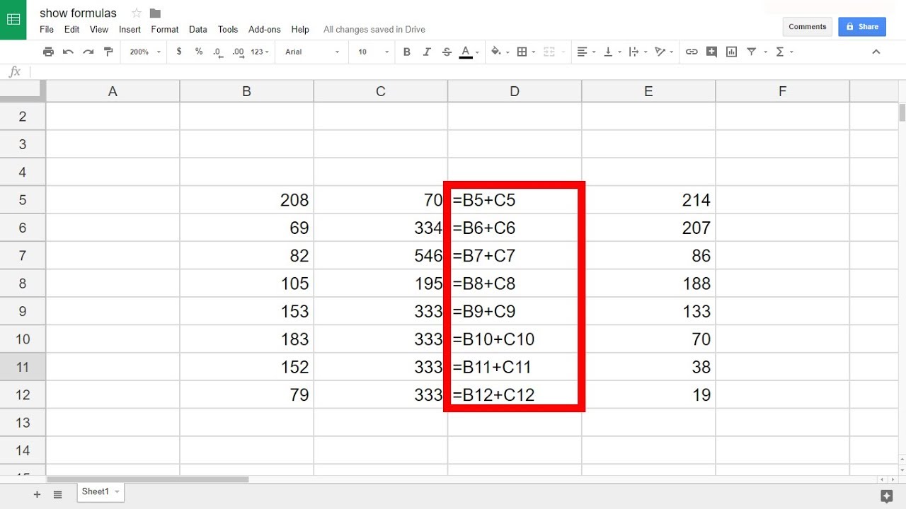
• ADDITION (+): To add two or more numbers together, you can simply use the plus sign (+) operator. For example, to add the values in cells A1 and B1, enter “=A1+B1” in a target cell.
• SUBTRACTION (-): To subtract one number from another, use the minus sign (-) operator. For instance, to subtract the value in cell B1 from cell A1, enter “=A1-B1” in a designated cell.
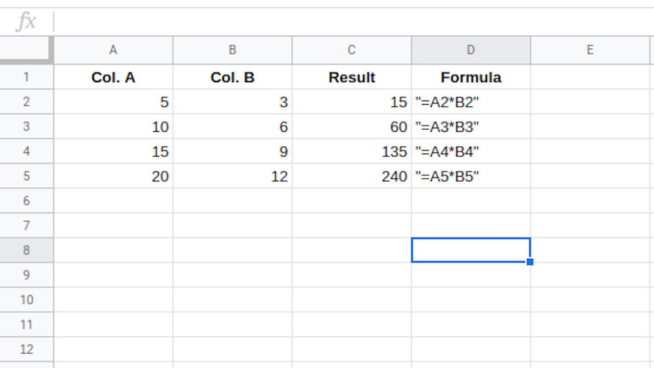
• MULTIPLICATION (*): To multiply two or more numbers together, utilize the asterisk (*) operator. For example, to multiply the values in cells A1 and B1, enter “=A1*B1” in a specific cell.
• DIVISION (/): To divide one number by another, use the forward slash (/) operator. For instance, to divide the value in cell A1 by cell B1, enter “=A1/B1” in a target cell.

In addition to these basic arithmetic operations, you can also use parentheses to control the order of operations. For example, if you want to add the sum of cells A1 and B1 to the product of cells C1 and D1, you can use parentheses like this: “= (A1+B1) + (C1*D1)”. This ensures that addition is performed before the multiplication.

Arithmetic formulas can be combined with other functions, such as SUM or AVERAGE, to perform more advanced calculations. For instance, you can find the total sales amount by using the formula “=SUM(A1:A10) * B1” where cells A1 to A10 contain sales quantities and cell B1 represents the price per unit.

By utilizing arithmetic formulas effectively in Google Sheets, you can automate calculations and save time on manual computations. These formulas are essential for performing numerical operations and are the foundation upon which more complex calculations can be built.

Now that you are familiar with arithmetic formulas, let’s explore the next set of formulas – logical formulas.

Logical Formulas

Logical formulas in Google Sheets are used to make comparisons and test conditions. These formulas evaluate whether certain conditions are true or false and perform different actions based on the result. Here are some commonly used logical formulas:

• EQUALS (==): The equals operator (==) checks if two values are equal. For example, to check if the value in cell A1 is equal to the value in cell B1, you can use the formula “=A1==B1”. This formula will return TRUE if the values are equal and FALSE otherwise.
• NOT EQUALS (!=): The not equals operator (!=) checks if two values are not equal. For instance, to check if the value in cell A1 is not equal to the value in cell B1, you can use the formula “=A1!=B1”. This formula will return TRUE if the values are not equal and FALSE otherwise.
• GREATER THAN (>), LESS THAN (<), GREATER THAN OR EQUAL TO (>=), LESS THAN OR EQUAL TO (<=): These operators are used to compare values. For example, to check if the value in cell A1 is greater than the value in cell B1, you can use the formula “=A1>B1”. Similarly, you can use “<", ">=”, and “<=" for other comparison operations.
• AND, OR: The AND and OR functions allow you to combine multiple conditions. The AND function returns TRUE if all conditions are true, while the OR function returns TRUE if at least one condition is true. These functions are useful for constructing complex logical expressions.
• IF: The IF function is a powerful tool for making decisions based on logical conditions. It allows you to specify different actions to take depending on whether a condition is true or false. For example, you can use the formula “=IF(A1>B1, “Yes”, “No”)” to check if the value in cell A1 is greater than the value in cell B1, and return “Yes” if true, and “No” if false.

Logical formulas are incredibly useful for data analysis and decision-making in Google Sheets. They can be used to filter and sort data, identify trends, automate tasks based on conditions, and much more.

By mastering logical formulas, you can make your spreadsheets more dynamic and responsive, allowing them to adapt to changing data and conditions. It’s a valuable skill for anyone who regularly works with large datasets or needs to perform complex calculations based on specific criteria.

Now that you understand logical formulas, let’s move on to exploring text formulas and how they can be used in Google Sheets.

Text Formulas

Text formulas in Google Sheets allow you to manipulate and combine text strings. These formulas are useful for formatting, extracting, and manipulating textual data in your spreadsheets. Here are some commonly used text formulas:

• CONCATENATE: The CONCATENATE function allows you to combine multiple text strings into one. For example, if you have the first name in cell A1 and the last name in cell B1, you can use the formula “=CONCATENATE(A1, ” “, B1)” to combine them with a space in between.
• LEFT, RIGHT, MID: These functions extract a portion of text from a cell. The LEFT function returns a specified number of characters from the beginning of a string, the RIGHT function returns a specified number of characters from the end, and the MID function returns a specified number of characters from any position within the string.
• LEN: The LEN function calculates the length of a text string. It returns the number of characters in a cell, including spaces and punctuation marks. This function is useful when you need to validate the length of certain text inputs or analyze the length of text strings in your data.
• LOWER, UPPER, PROPER: These functions allow you to change the case of text. LOWER converts all text to lowercase, UPPER converts all text to uppercase, and PROPER capitalizes the first letter of each word in a text string.
• TRIM: The TRIM function removes leading and trailing spaces from a text string. It is useful when you have imported or copied text that contains unnecessary spaces.

Text formulas can be combined with other formulas and functions to perform more complex operations. For example, you can use the CONCATENATE function to combine text strings with the results of arithmetic or logical formulas, or with the results of functions like TODAY() or NOW() to generate dynamic text.

By utilizing text formulas effectively in Google Sheets, you can format and manipulate text strings to suit your needs. Whether you’re working with names, addresses, product descriptions, or any other textual data, these formulas will help you streamline your processes and enhance the consistency of your spreadsheets.

Now that you have an understanding of text formulas, let’s explore how to work with dates and times in Google Sheets.

Date and Time Formulas

Date and time formulas in Google Sheets allow you to work with and manipulate dates and times within your spreadsheets. These formulas are vital for tracking deadlines, calculating durations, and performing various operations based on specific dates and times. Here are some commonly used date and time formulas:

• TODAY: The TODAY function returns the current date. This formula is useful for automatically updating cells with the current date whenever the spreadsheet is opened or recalculated.
• NOW: The NOW function returns the current date and time. This formula is helpful for tracking events and recording the exact time of data entry or calculations.
• DATE: The DATE function allows you to create a date by specifying the year, month, and day. For example, to create the date January 1, 2022, you can use the formula “=DATE(2022, 1, 1)”.
• DAY, MONTH, YEAR: These functions extract the day, month, or year from a given date. For instance, the DAY function returns the day of the month for a specified date, the MONTH function returns the month, and the YEAR function returns the year.
• DATEDIF: The DATEDIF function calculates the difference between two dates in terms of days, months, or years. This formula is useful for determining the duration between two events or calculating an individual’s age.
• EDATE, EOMONTH: The EDATE function adds or subtracts a specified number of months from a given date. The EOMONTH function returns the last day of a specific month, either in the past or future. These functions are handy for managing deadlines and projecting future dates.

Date and time formulas can be combined with other formulas and functions to perform more advanced calculations. For example, you can use the DATEDIF function to calculate the age of a person by subtracting their birthdate from the current date provided by the TODAY function.

By understanding and utilizing date and time formulas effectively in Google Sheets, you can keep track of important events, calculate durations accurately, and ensure timely completion of tasks.

Now that you have a grasp of date and time formulas, let’s explore how to use conditional formulas in Google Sheets.

Conditional Formulas

Conditional formulas in Google Sheets allow you to perform calculations or display specific values based on certain conditions. These formulas evaluate a particular criterion or set of criteria and return results accordingly. Conditional formulas are crucial for automating data analysis and making decisions based on specific conditions. Here are some commonly used conditional formulas:

• IF: The IF function is one of the most versatile conditional formulas. It allows you to specify different outcomes based on a logical condition. For example, you can use the formula “=IF(A1>10, “Yes”, “No”)” to check if the value in cell A1 is greater than 10. If it is, the formula will return “Yes”, otherwise, it will return “No”.
• AND, OR: The AND and OR functions are used to evaluate multiple conditions. The AND function returns TRUE if all conditions are true, while the OR function returns TRUE if at least one condition is true. These functions are useful when you need to check multiple criteria simultaneously.
• ISBLANK, ISNOTBLANK: These functions are used to check if a cell is empty (ISBLANK) or not empty (ISNOTBLANK). They are handy for validating data entry or determining if a cell contains a value.
• COUNTIF, SUMIF, AVERAGEIF: These functions allow you to perform calculations based on specific criteria. COUNTIF counts the number of cells that meet a certain condition, SUMIF sums the values of cells that meet a certain condition, and AVERAGEIF calculates the average of cells that meet a certain condition.
• Nested IF: You can also nest multiple IF functions within each other to create more complex conditional statements. This is useful when you have multiple conditions that need to be evaluated in a specific order.

Conditional formulas can be combined with other formulas and functions to perform more sophisticated calculations and automate decision-making processes. They are invaluable for filtering data, highlighting specific values, and generating dynamic reports based on specific criteria.

By mastering conditional formulas in Google Sheets, you can streamline your data analysis and make your spreadsheets more responsive to changing conditions. They provide a powerful tool for automating tasks and generating accurate, customized reports based on specific criteria.

Now that you understand conditional formulas, let’s explore how to use lookup formulas in Google Sheets.

Lookup Formulas

Lookup formulas in Google Sheets allow you to search for specific values in a dataset and retrieve related information. These formulas are useful for locating data from a different sheet or within the same sheet based on certain criteria. Lookup formulas enable you to find, match, and retrieve data efficiently. Here are some commonly used lookup formulas:

• VLOOKUP: The VLOOKUP function searches for a value in the leftmost column of a range and returns a corresponding value from a specified column. It is particularly useful when you have a large dataset and need to find specific information based on a unique identifier.
• HLOOKUP: Similar to VLOOKUP, the HLOOKUP function searches for a value in the top row of a range and returns a corresponding value from a specified row. This is handy when you want to search horizontally rather than vertically.
• INDEX/MATCH: The INDEX and MATCH functions are often used together to perform more advanced lookups. The INDEX function returns a value based on a given row and column number, while the MATCH function searches for a value in a range and returns its position. Together, these functions enable you to flexibly search and retrieve data based on multiple criteria.

Lookup formulas are highly versatile and can be combined with other functions to refine the search and retrieve specific information. They are beneficial for managing large datasets, creating reports, and conducting data analysis.

By mastering lookup formulas in Google Sheets, you can greatly enhance your ability to locate and retrieve relevant data quickly and accurately. They provide powerful tools for data manipulation and data-driven decision-making.

Now that you understand lookup formulas, let’s explore another powerful feature in Google Sheets – array formulas.

Array Formulas

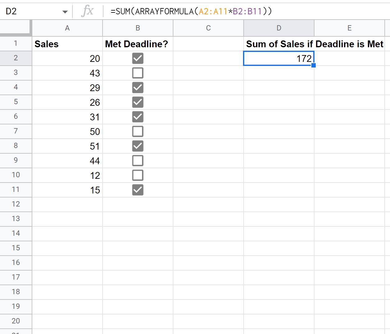
Array formulas in Google Sheets allow you to perform calculations on multiple cells at once and return an array or a range of values as the result. These formulas are powerful tools for analyzing complex data and performing calculations that would otherwise require multiple individual formulas. Array formulas can be used to manipulate large datasets, perform calculations across multiple rows and columns, and produce dynamic results. Here are some key points about array formulas:

• Single-cell array formulas: In some cases, array formulas can be used in a single cell, but they perform calculations on a range of cells. The formula is entered into the cell, surrounded by curly braces ({ }), to indicate that it is an array formula. The result of the array formula is displayed in that cell, but it actually affects the entire range specified in the formula.
• Advantages of array formulas: Array formulas can perform complex calculations with minimal formulas and reduce the need for additional helper columns. They can process large data sets efficiently and provide dynamic results that update automatically when the underlying data changes.
• Common array formulas: Common use cases of array formulas include summing a range of values that meet multiple criteria, finding the largest or smallest value in a range, performing calculations on filtered data, and transposing or flipping data orientation.
• Cautions: Array formulas can be more resource-intensive than regular formulas and can slow down spreadsheet performance, especially if used extensively. It is important to be cautious when using array formulas with very large data sets.

Array formulas provide a powerful way to perform advanced calculations and manipulate data in Google Sheets. By mastering array formulas, you can streamline your calculations, enhance the efficiency of your spreadsheets, and gain deeper insights from your data.

Now that you have an overview of array formulas, let’s move on to some helpful tips and tricks to make the most out of formulas in Google Sheets.

Formula Tips and Tricks

Mastering formulas in Google Sheets can greatly improve your productivity and efficiency. To help you make the most out of formulas, here are some valuable tips and tricks:

• Understand cell references: It’s crucial to understand how cell references work in formulas. Use absolute references with dollar signs ($A$1) when you want a reference to remain constant when copying the formula, and use relative references (A1) when you want the reference to adjust automatically.
• Use named ranges: Named ranges make formulas easier to read and understand. Instead of using cell references, you can assign names to specific ranges and use those names in your formulas. This makes your formulas more intuitive and reduces the chances of errors when referencing cells.
• Utilize function arguments: Many functions in Google Sheets have optional arguments that can modify their behavior. Take some time to explore the available arguments and customize the functions to fit your specific needs, such as formatting options or additional criteria.
• Format your formulas: Adding line breaks, indentations, and comments within your formulas can make them more readable and easier to troubleshoot. Use spaces and formatting to visually separate different parts of your formulas and improve clarity.
• Use data validation: Data validation can help prevent errors and ensure accurate data entry. You can set up custom rules to restrict the input in cells and guide users to enter valid data, reducing the risk of formula errors.
• Explore built-in templates: Google Sheets offers a wide range of pre-built templates that include formulas specific to different use cases. Take advantage of these templates as a starting point for your projects, and modify them to suit your needs.
• Stay organized: Keep your formulas organized by using different sheets or tabs within your spreadsheet. You can group related data and formulas together, making it easier to navigate and maintain large files.

By implementing these tips and tricks, you can streamline your workflow, reduce errors, and improve the efficiency and effectiveness of your formulas in Google Sheets.

Now that you have a solid foundation in using formulas and are equipped with these helpful tips, you can confidently tackle data analysis, automate tasks, and unlock the full potential of Google Sheets.

Conclusion

Formulas are the backbone of Google Sheets, allowing you to perform complex calculations, manipulate data, and automate tasks. By mastering the various types of formulas, you can unlock the full potential of this powerful tool and enhance your productivity in organizing and analyzing data.

In this article, we covered the essential formulas in Google Sheets, starting with the basic arithmetic formulas that enable you to perform simple calculations. We then explored logical formulas, which help you make comparisons and test conditions based on logical expressions. Text formulas allow you to manipulate and combine text strings, while date and time formulas enable you to work with dates and times, performing calculations and tracking events effectively.

Conditional formulas help you make decisions and perform actions based on specific conditions, while lookup formulas allow you to search for values and retrieve related information from datasets. Finally, we explored array formulas, which provide powerful tools for performing calculations on multiple cells at once and generating dynamic results.

To make the most out of formulas, we shared valuable tips and tricks, including understanding cell references, using named ranges, customizing function arguments, formatting formulas for readability, implementing data validation, exploring built-in templates, and staying organized within your spreadsheet.

By applying these techniques and continuously practicing with formulas, you can become more proficient in Google Sheets and streamline your data analysis and manipulation. Formulas not only save you time and effort but also enable you to gain valuable insights and make data-driven decisions.

So, take the knowledge you have gained from this article and start exploring the endless possibilities of formulas in Google Sheets. With practice and experimentation, you can become a skilled user, leveraging formulas to optimize your workflows and achieve your goals.