Introduction
Google Sheets is a powerful and versatile tool for creating and managing spreadsheets online. Whether you are a student, a professional, or a small business owner, understanding how to use formulas in Google Sheets can greatly enhance your productivity and efficiency.
Formulas in Google Sheets allow you to perform calculations, manipulate data, and automate tasks. With a wide range of built-in functions, you can easily perform complex mathematical calculations, analyze data statistically, process text, and work with dates and times.
In this article, we will guide you through the process of adding formulas in Google Sheets. We will cover the basics of creating a new Google Sheets document, entering data, and understanding the different types of formulas available. We will also explore common mathematical formulas, statistical and analytical formulas, logical functions, text functions, and date and time functions.
By the end of this article, you will have a solid understanding of how to use formulas in Google Sheets and will be equipped with the knowledge to perform various calculations and analysis. Whether you need to calculate sales figures, analyze survey data, or automate repetitive tasks, mastering formulas in Google Sheets will unlock a whole new level of productivity and efficiency.
So, let’s dive in and explore the world of formulas in Google Sheets!
Creating a New Google Sheets Document
To get started with using formulas in Google Sheets, the first step is to create a new Google Sheets document. Follow these simple steps:
- Open your web browser and go to Google Sheets.
- If you have a Google account, sign in. If not, you can create a Google account for free.
- Click on the “+ New” button to create a new document. A drop-down menu will appear.
- Select “Google Sheets” from the menu. A blank Google Sheets document will open.
- Give your document a meaningful title by clicking on the current document name at the top-left corner and typing a new name.
That’s it! You now have a new Google Sheets document ready to be filled with data and formulas.
In Google Sheets, a document consists of different sheets, similar to the tabs in a physical binder. By default, a new document is created with one sheet, but you can add more sheets as needed. Each sheet can contain multiple rows and columns, forming a grid where you can enter and manipulate data.
With the basic setup complete, let’s move on to the next section and learn how to enter data in Google Sheets.
Entering Data in Google Sheets
Now that you have created a new Google Sheets document, it’s time to enter data into the spreadsheet. Follow these steps to enter data in Google Sheets:
- Click on the first cell of the sheet, typically cell A1, to select it. The selected cell will be highlighted.
- Type the desired data into the selected cell. You can enter text, numbers, or a combination of both.
- Press Enter on your keyboard to move to the next cell in the same column. Alternatively, you can use the Tab key to move to the next cell in the same row.
- Continue entering data into the cells following the same process.
You can also copy and paste data from another source, such as a spreadsheet or a text document, into Google Sheets. To do this, select the data you want to copy, press Ctrl+C (or Command+C on Mac) to copy, click on the destination cell in Google Sheets, and press Ctrl+V (or Command+V on Mac) to paste.
In addition to entering data manually, there are other methods to populate a large amount of data quickly. For example, you can drag the fill handle to automatically fill a series or pattern of data in adjacent cells. This is particularly useful when entering dates, numbers, or any repeating pattern.
Furthermore, you can use the “Import” function to bring data from other sources, such as CSV files, Excel spreadsheets, or webpages. Google Sheets allows you to import data seamlessly, making it easy to work with data from different sources.
Entering and managing data is the foundation of any spreadsheet. With your data entered into Google Sheets, you are now ready to explore the world of formulas and unleash the true power of this versatile tool.
Understanding Basic Formulas in Google Sheets
Formulas are the heart and soul of Google Sheets. They allow you to perform calculations and manipulate data dynamically. Understanding the basics of formulas is essential to effectively use Google Sheets. Here are a few key concepts to get you started:
1. Formula Syntax: A formula in Google Sheets begins with an equals sign (=) followed by the expression to be evaluated. For example, =A1+B1 calculates the sum of the values in cells A1 and B1.
2. Operators: Google Sheets supports a variety of mathematical operators to perform calculations. Basic arithmetic operators include addition (+), subtraction (-), multiplication (*), and division (/). Additional operators include exponentiation (^), percent (%), and concatenation (&).
3. Cell References: In a formula, you can refer to specific cells by their column and row coordinates. For example, A1 refers to the cell in column A and row 1. The use of cell references allows formulas to dynamically update when the referenced cells change.
4. Built-in Functions: Google Sheets provides a wide range of built-in functions to perform specific calculations. Functions can be used in formulas to perform complex calculations or manipulate data. For example, the SUM function calculates the sum of a range of cells: =SUM(A1:A10).
5. Auto-fill: Google Sheets has a handy feature called Auto-fill that can automatically extend formulas to adjacent cells. This is particularly useful when working with a large dataset or when copying formulas to multiple cells.
By understanding these basic concepts, you can start creating simple formulas to perform calculations in Google Sheets. In the next section, we will delve deeper into adding formulas and explore the different types of formulas available in Google Sheets.
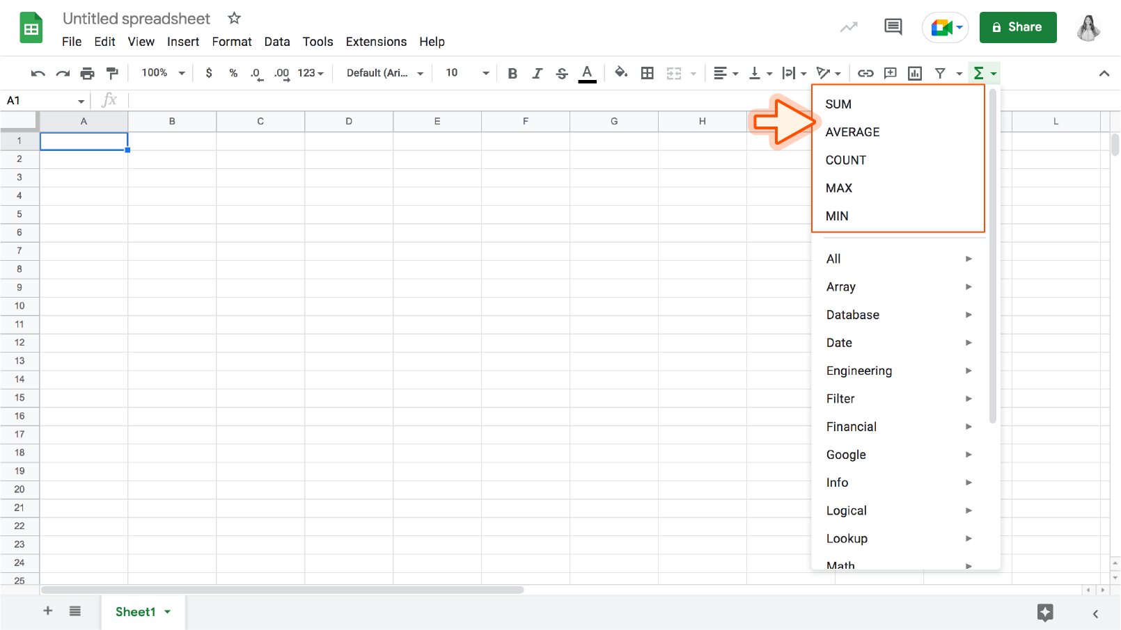
Adding Formulas in Google Sheets
Adding formulas in Google Sheets is a straightforward process that allows you to perform calculations and manipulate data dynamically. To add a formula, follow these steps:
- Select the cell where you want the formula result to appear.
- Type an equals sign (=) to indicate the start of a formula.
- Enter the formula, using appropriate operators, cell references, and/or functions.
- Press Enter on your keyboard to apply the formula to the selected cell.
When you press Enter, Google Sheets will calculate the formula and display the result in the selected cell. You can then copy the formula to other cells by dragging the fill handle, or you can use the Auto-fill feature to automatically extend the formula to adjacent cells.
It’s important to note that Google Sheets follows the order of operations (PEMDAS/BODMAS) when evaluating formulas. This means that calculations inside parentheses are performed first, followed by exponents, multiplication and division (from left to right), and finally addition and subtraction (from left to right).
Google Sheets also supports a wide range of functions that can be used in formulas to perform specific calculations or manipulate data. These functions can range from simple arithmetic functions like SUM and AVERAGE to more complex statistical, logical, text, and date functions.
Additionally, you can use cell references in formulas to dynamically refer to the values in other cells. This allows your formulas to update automatically when the referenced cells change.
By combining operators, functions, and cell references, you can create powerful and flexible formulas in Google Sheets to perform various calculations and manipulate your data effectively.
In the following sections, we will explore different types of formulas available in Google Sheets, including common mathematical formulas, statistical and analytical formulas, logical functions, text functions, and date and time functions.
Common Mathematical Formulas in Google Sheets
Google Sheets provides a wide range of mathematical formulas and functions that allow you to perform basic to advanced calculations on your data. Here are some of the common mathematical formulas you can use in Google Sheets:
1. SUM: The SUM formula is used to calculate the sum of a range of cells. For example, =SUM(A1:A10) will add up the values in cells A1 to A10.
2. AVERAGE: The AVERAGE formula calculates the average value of a range of cells. For example, =AVERAGE(B1:B10) will give you the average of the values in cells B1 to B10.
3. MAX and MIN: The MAX and MIN formulas determine the highest and lowest values in a range of cells, respectively. For example, =MAX(C1:C5) will return the maximum value in cells C1 to C5.
4. COUNT: The COUNT formula counts the number of cells in a range that contain numerical values. For example, =COUNT(D1:D10) will give you the count of cells in range D1 to D10 that contain numbers.
5. SQRT: The SQRT formula calculates the square root of a number. For example, =SQRT(E1) will give you the square root of the value in cell E1.
6. POWER: The POWER formula raises a number to a specified power. For example, =POWER(F1, 2) will raise the value in cell F1 to the power of 2.
7. ROUND: The ROUND formula rounds a number to a specified number of decimal places. For example, =ROUND(G1, 2) will round the value in cell G1 to 2 decimal places.
8. RAND: The RAND formula generates a random number between 0 and 1. For example, =RAND() will give you a random number each time the sheet recalculates.
These are just a few examples of the mathematical formulas available in Google Sheets. You can explore the built-in functions library to find more advanced mathematical formulas and functions for your specific needs.
Now that you have an understanding of the common mathematical formulas, let’s move on to the next section and explore statistical and analytical formulas in Google Sheets.
Statistical and Analytical Formulas in Google Sheets
Google Sheets offers a range of statistical and analytical formulas that allow you to analyze and summarize your data. These formulas can help you gain insights, make informed decisions, and uncover patterns and trends in your data. Here are some of the key statistical and analytical formulas available in Google Sheets:
1. COUNTIFS: The COUNTIFS formula counts the number of cells that meet multiple criteria. For example, =COUNTIFS(A1:A10, “>50”, B1:B10, “<100") will count the number of cells in the range A1:A10 that are greater than 50 and in the range B1:B10 that are less than 100.
2. AVERAGEIFS: The AVERAGEIFS formula calculates the average of cells that meet multiple criteria. For example, =AVERAGEIFS(C1:C10, A1:A10, “Apples”, B1:B10, “Red”) will give you the average value in the range C1:C10 for cells that have “Apples” in column A and “Red” in column B.
3. SUMIFS: The SUMIFS formula calculates the sum of cells that meet multiple criteria. For example, =SUMIFS(D1:D10, A1:A10, “Bananas”, B1:B10, “Yellow”) will give you the sum of values in the range D1:D10 for cells that have “Bananas” in column A and “Yellow” in column B.
4. MAXIFS and MINIFS: The MAXIFS and MINIFS formulas allow you to find the maximum and minimum values that meet multiple criteria, respectively. For example, =MAXIFS(E1:E10, A1:A10, “Oranges”, B1:B10, “Orange”) will return the maximum value in the range E1:E10 for cells that have “Oranges” in column A and “Orange” in column B.
5. COUNTA: The COUNTA formula counts the number of non-empty cells in a range. For example, =COUNTA(F1:F10) will count the number of non-empty cells in the range F1 to F10.
6. MEDIAN: The MEDIAN formula calculates the median value of a range of cells. For example, =MEDIAN(G1:G10) will give you the median value of the range G1 to G10.
7. CORR: The CORR formula calculates the correlation coefficient between two ranges of cells, which indicates the relationship between them. For example, =CORR(H1:H10, I1:I10) will return the correlation coefficient between the ranges H1 to H10 and I1 to I10.
These are just a few examples of the statistical and analytical formulas available in Google Sheets. You can explore the built-in functions library to find more formulas that suit your data analysis needs.
Next, we will explore the use of logical functions in Google Sheets and see how they can help you evaluate conditions and make logical decisions based on your data.
Using Logical Functions in Google Sheets
Logical functions in Google Sheets allow you to evaluate conditions and perform logical operations on your data. These functions can help you make decisions, filter data, and perform complex calculations based on specific criteria. Here are some commonly used logical functions in Google Sheets:
1. IF: The IF function is a powerful tool for making logical decisions in Google Sheets. It allows you to specify a condition and provides different results based on whether the condition is true or false. For example, =IF(A1>10, “Yes”, “No”) will check if the value in cell A1 is greater than 10. If it is, the formula will return “Yes”, otherwise it will return “No”.
2. AND: The AND function evaluates multiple conditions and returns true only if all the conditions are true. For example, =AND(A1>10, B1<20) will check if both the value in cell A1 is greater than 10 and the value in cell B1 is less than 20. If both conditions are true, the formula will return true, otherwise it will return false.
3. OR: The OR function evaluates multiple conditions and returns true if any of the conditions are true. For example, =OR(A1>10, B1<20) will check if either the value in cell A1 is greater than 10 or the value in cell B1 is less than 20. If at least one of the conditions is true, the formula will return true, otherwise it will return false.
4. NOT: The NOT function negates a logical value. It returns true if the logical value is false, and false if the logical value is true. For example, =NOT(A1=10) will check if the value in cell A1 is not equal to 10. If it is not equal, the formula will return true, otherwise it will return false.
5. IFERROR: The IFERROR function allows you to handle errors in your formulas. It checks for an error and provides an alternate value or action if an error occurs. For example, =IFERROR(A1/B1, “Error”) will calculate the result of dividing the value in cell A1 by the value in cell B1. If an error occurs (e.g., when dividing by zero), the formula will return “Error”.
By using these logical functions, you can create dynamic formulas that make logical decisions, perform complex calculations, and filter data based on specific criteria. Understanding and leveraging these functions can greatly enhance your data analysis capabilities in Google Sheets.
Next, let’s explore how to work with text functions in Google Sheets, which can help you manipulate and analyze text data efficiently.
Working with Text Functions in Google Sheets
Text functions in Google Sheets allow you to manipulate and analyze text data effectively. Whether you need to extract specific information from a string, combine text from multiple cells, or format text in a specific way, these functions can help you achieve your desired results. Here are some commonly used text functions in Google Sheets:
1. CONCATENATE: The CONCATENATE function allows you to combine multiple text strings into one. For example, =CONCATENATE(A1, ” “, B1) will concatenate the text in cell A1 with a space and the text in cell B1.
2. LEFT and RIGHT: The LEFT function extracts a specified number of characters from the beginning of a text string, while the RIGHT function extracts a specified number of characters from the end. For example, =LEFT(C1, 3) will extract the leftmost three characters from the text in cell C1.
3. MID: The MID function extracts a specified number of characters from a text string, starting at a given position. For example, =MID(D1, 2, 4) will extract four characters from the text in cell D1, starting at the second character.
4. LEN: The LEN function returns the length of a text string, including spaces and special characters. For example, =LEN(E1) will give you the number of characters in the text in cell E1.
5. LOWER and UPPER: The LOWER function converts a text string to lowercase, while the UPPER function converts it to uppercase. For example, =LOWER(F1) will convert the text in cell F1 to lowercase.
6. SUBSTITUTE: The SUBSTITUTE function replaces occurrences of a specific text within a larger text string. For example, =SUBSTITUTE(G1, “old”, “new”) will replace the word “old” with the word “new” in the text in cell G1.
7. FIND and SEARCH: The FIND function and the SEARCH function both search for a specified text within a larger text string. The difference is that FIND is case-sensitive, while SEARCH is not. These functions return the position at which the search text is found. For example, =FIND(“search”, H1) will give you the position of the word “search” within the text in cell H1.
By using these text functions, you can manipulate and analyze text data in a variety of ways, such as extracting specific information, combining text strings, formatting text, and more. These functions are invaluable when working with textual data in Google Sheets.
Now, let’s move on to the next section and explore how to work with date and time functions in Google Sheets.
Date and Time Functions in Google Sheets
Date and time functions in Google Sheets allow you to work with dates, times, and time intervals in various ways. Whether you need to calculate the number of days between two dates, extract the day of the week from a date, or format dates and times in a specific way, these functions can help you handle your date and time data effectively. Here are some commonly used date and time functions in Google Sheets:
1. TODAY and NOW: The TODAY function returns the current date, while the NOW function returns the current date and time. These functions are dynamic and update automatically when the sheet recalculates.
2. DATE: The DATE function allows you to create a date based on specified year, month, and day values. For example, =DATE(2022, 4, 15) will return the date April 15, 2022.
3. YEAR, MONTH, DAY: The YEAR, MONTH, and DAY functions extract the year, month, and day from a given date, respectively. For example, =YEAR(A1) will give you the year of the date in cell A1.
4. DATEDIF: The DATEDIF function calculates the difference between two dates in terms of years, months, or days. For example, =DATEDIF(B1, C1, “Y”) will give you the number of complete years between the dates in cells B1 and C1.
5. WEEKDAY: The WEEKDAY function returns the day of the week for a given date as a number, where Sunday is 1 and Saturday is 7. For example, =WEEKDAY(D1) will give you the day of the week for the date in cell D1.
6. EDATE and EOMONTH: The EDATE function adds or subtracts a specified number of months from a given date. The EOMONTH function returns the last day of the month for a given date. For example, =EDATE(E1, 6) will give you the date that is 6 months after the date in cell E1, and =EOMONTH(F1, 0) will give you the last day of the month for the date in cell F1.
7. TIME: The TIME function allows you to create a time value based on specified hour, minute, and second values. For example, =TIME(9, 30, 0) will return the time 9:30:00 AM.
These date and time functions in Google Sheets provide powerful tools to work with your date and time data. Whether you need to perform calculations, extract specific information, or format dates and times, these functions can help you accomplish your tasks efficiently.
Now that you have an understanding of the date and time functions, let’s move on to some tips and tricks for working with formulas effectively in Google Sheets.
Tips and Tricks for Working with Formulas in Google Sheets
Working with formulas in Google Sheets can be made easier and more efficient with a few tips and tricks. Here are some strategies to help you navigate and maximize your use of formulas:
1. Use cell references: Instead of entering static values in your formulas, use cell references to dynamically refer to the data in other cells. This allows your formulas to update automatically when the referenced cells change.
2. Leverage auto-fill: Use the fill handle to quickly copy formulas to adjacent cells. You can drag the fill handle to fill a series or pattern of formulas. This is especially useful in situations where you have a large dataset or need to replicate formulas across multiple cells.
3. Be mindful of parentheses: When using complex formulas with multiple operations, make sure to use parentheses to specify the order in which the operations should be performed. This helps avoid confusion and ensures accurate calculations.
4. Explore the built-in functions: Google Sheets offers a vast library of built-in functions. Take the time to explore and familiarize yourself with the various functions available. These functions can save you time and effort by providing ready-made solutions for specific calculations or data manipulations.
5. Use named ranges: Assigning a name to a range of cells can make your formulas more readable and easier to understand. Instead of using cell references, you can refer to named ranges in your formulas, resulting in more intuitive and concise formulas.
6. Check for errors: Always double-check your formulas for any errors. Google Sheets provides error checking tools that can help you detect and resolve formula errors, such as missing parentheses, incorrect cell references, or invalid functions.
7. Utilize formatting options: Formatting your cells can enhance the visual clarity of your spreadsheet. Apply number formats, font styles, and cell borders to improve readability and distinguish different types of data in your formulas.
8. Document your formulas: Adding comments or annotations to your formulas can make your spreadsheet more understandable and maintainable. Documenting the purpose and logic of your formulas can help you and others interpret and troubleshoot the spreadsheet in the future.
By implementing these tips and tricks, you can become more proficient and efficient in working with formulas in Google Sheets. These strategies will help you streamline your workflow, improve the accuracy of your calculations, and enhance the overall usability of your spreadsheets.
Now that you’re equipped with these practical tips, you’re ready to harness the full potential of working with formulas in Google Sheets.
Conclusion
Formulas are an indispensable tool in Google Sheets, allowing you to perform complex calculations, analyze data, and automate tasks. By mastering formulas, you can unlock the full potential of this powerful spreadsheet application. Throughout this article, we have covered the essential steps for creating a new Google Sheets document, entering data, and understanding the basics of formulas.
We explored a range of formulas, including common mathematical formulas, statistical and analytical formulas, logical functions, text functions, and date and time functions. These functions provide the flexibility to manipulate and analyze your data in various ways, enabling you to derive meaningful insights and make informed decisions.
Additionally, we provided practical tips and tricks to enhance your formula usage in Google Sheets. By leveraging features like cell references, auto-fill, and named ranges, you can streamline your workflow and increase your efficiency. Paying attention to formatting, error checking, and documenting your formulas ensures accuracy and maintainability in your spreadsheet projects.
As you continue to explore and experiment with formulas in Google Sheets, keep in mind the vast capabilities and possibilities they offer. With practice and familiarity, you will become more proficient in utilizing formulas to solve complex problems, automate repetitive tasks, and present data in a clear and meaningful way.
Remember, formulas are not only about calculations, but also about presenting information effectively. Balancing the use of formulas with clear data visualization and thoughtful organization will result in compelling and comprehensible spreadsheets.
So, whether you are a student, a professional, or a small business owner, investing time in understanding and mastering formulas in Google Sheets will undoubtedly enhance your productivity and efficiency. Embrace the power of formulas and unlock a world of possibilities within your spreadsheets.