How To Make A Row Stay In Google Sheets

Introduction

Google Sheets is a powerful spreadsheet tool that offers a wide range of features for organizing and analyzing data. However, when working with large datasets or complex spreadsheets, it can sometimes be challenging to keep important information in view while scrolling through rows and columns. One common issue users face is how to make a particular row stay visible as they navigate through the sheet.

In this article, we will explore several methods to help you keep a row visible in Google Sheets. Whether you need to keep headers, summary information, or any other critical row fixed in view, these methods will save you time and effort in locating and referencing important data.

We will cover five different techniques that range from simple to more advanced, each with its own advantages and use cases. By utilizing these methods, you can customize your Google Sheets experience and improve your productivity when working with large datasets or complex spreadsheets.

So, let’s dive in and discover how to make a row stay in Google Sheets!

Method 1: Freeze Panes

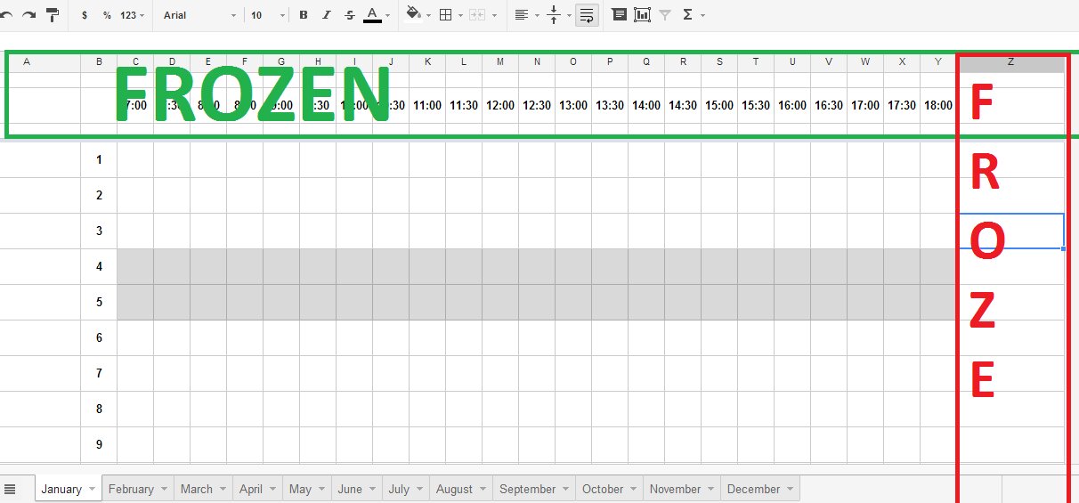
One of the easiest and most straightforward ways to make a row stay visible in Google Sheets is by using the “Freeze Panes” feature. This feature allows you to freeze a specific row or column so that it remains visible even when scrolling through your spreadsheet.

To freeze a row, follow these steps:

1. Select the row below the one you want to freeze. For example, if you want to freeze row 1, select cell A2.
2. Click on the “View” menu at the top.
3. Hover over the “Freeze” option.
4. Select “1 row” from the submenu.

Once you’ve completed these steps, the selected row, in this case, row 1, will be frozen, and you can scroll through the rest of your spreadsheet while still keeping that row visible at the top.

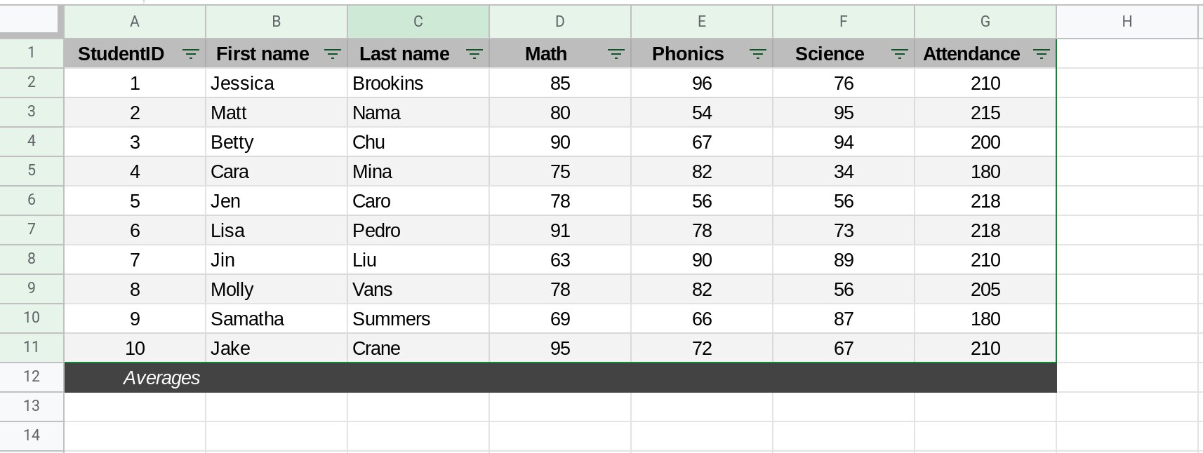
This method is especially useful when you have headers or labels in the first row that you need to reference while working on other parts of your spreadsheet. Freezing the row ensures that the labels are always visible, providing constant context for your data without the need for constant scrolling up and down.

It’s important to note that you can also freeze multiple rows or columns by selecting the appropriate number of rows or columns before accessing the “Freeze” menu. This flexibility allows you to tailor the freezing feature to your specific worksheet layout and requirements.

Overall, the “Freeze Panes” feature is a simple yet effective method to make a row stay visible in Google Sheets. By utilizing this feature, you can streamline your workflow and significantly improve your productivity when working with complex spreadsheets.

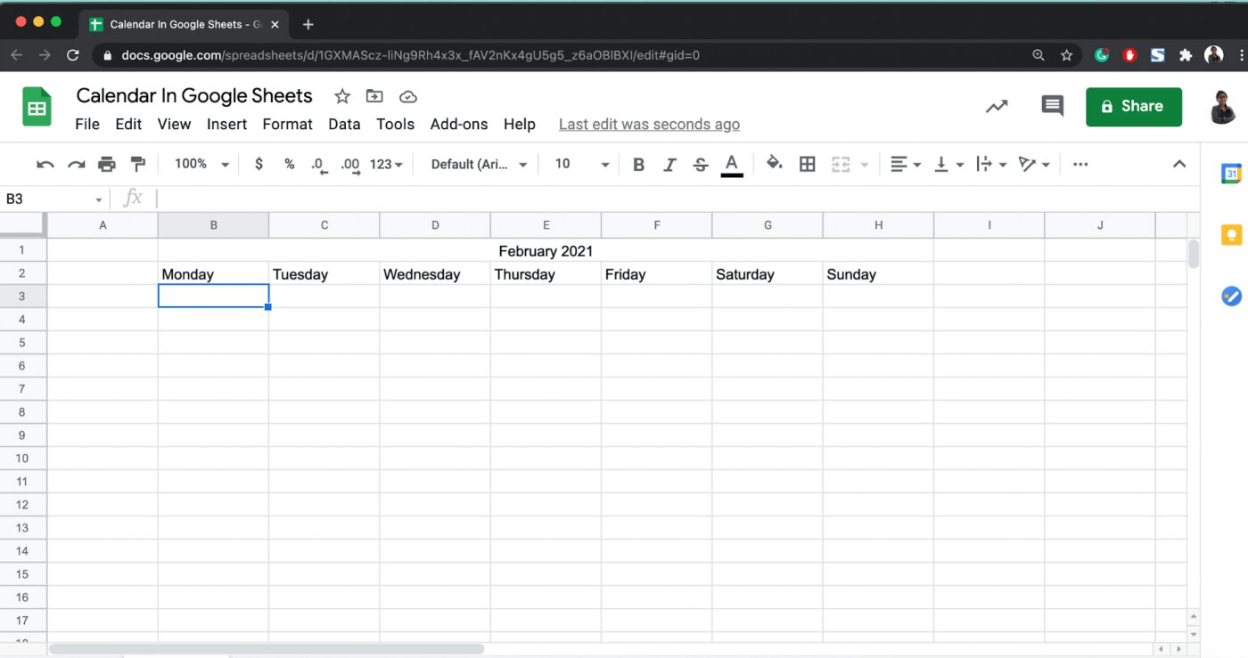
Method 2: Split View

If you want to keep a row visible without freezing it in place, Google Sheets offers a feature called “Split View”. Split View allows you to create separate, resizable views of your spreadsheet, making it easier to keep track of specific rows or columns as you navigate through your data.

To use the Split View feature in Google Sheets, follow these steps:

1. Open your spreadsheet in Google Sheets.
2. Click on the “View” menu at the top.
3. Hover over the “Split” option.
4. Select either “Vertical split” or “Horizontal split” based on your preference.

After splitting the view, you will notice two separate windows within the same spreadsheet. You can then adjust the divider between the windows to customize the size of each view.

To keep a specific row visible, position the divider so that the row you want to keep visible is in one view, while the rest of the spreadsheet can be accessed in the other view.

This method is particularly useful when you need to compare data from different rows side by side, or when you want to keep a summary row visible while working on other parts of your spreadsheet. The Split View feature allows you to multitask more efficiently and eliminates the need for constant scrolling or manual freezing.

It’s worth noting that you can have multiple split views by repeating the steps above. This flexibility enables you to create customized views that suit your specific data analysis needs.

By using the Split View feature in Google Sheets, you can keep a row visible while still navigating through your spreadsheet effortlessly, improving your data analysis workflow and productivity.

Method 3: Use a Helper Column

If you prefer a more hands-on approach to keep a row visible in Google Sheets, you can utilize a helper column. A helper column is an additional column added to your spreadsheet that contains a specific formula or value to assist in achieving your desired outcome.

To use a helper column to keep a row visible, follow these steps:

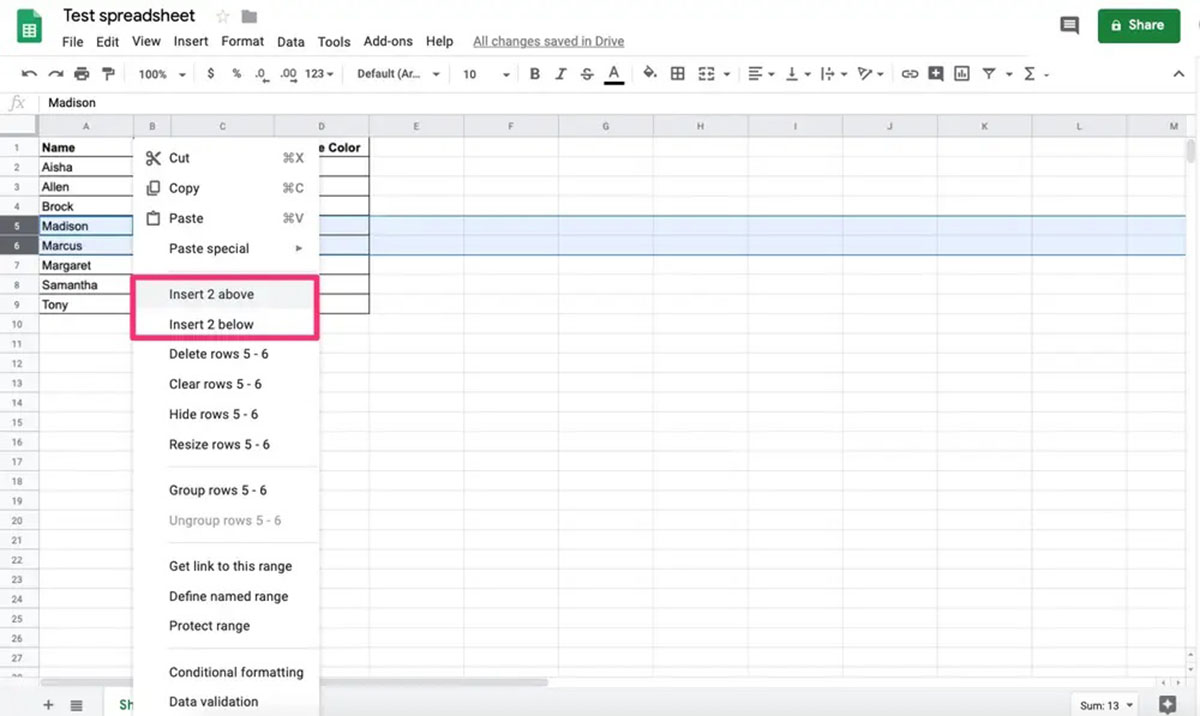
1. Identify an empty column next to your data.
2. Click on the first cell in the helper column.
3. Enter a formula or value that references the desired row you want to keep visible.
4. Drag the formula or value down to apply it to the entire column.

The helper column acts as a reference point, allowing you to quickly locate and keep track of the desired row as you navigate through your spreadsheet. With the help of this column, you can easily identify the corresponding row based on the values or formulas you inputted.

This method is especially useful when you have specific criteria to determine which rows should stay visible. For example, you can use conditional formatting or logical functions such as IF or COUNTIF to make the helper column dynamically update based on certain conditions or calculations.

By utilizing a helper column, you have more control over which row to keep visible, even if the data in your spreadsheet changes. This method gives you the flexibility to adapt to varying scenarios and ensures you always have the necessary information at your fingertips.

Remember to hide or adjust the width of the helper column if you don’t want it to be visible in your final presentation or analysis.

Using a helper column enables you to customize the visibility of specific rows in Google Sheets, providing a practical solution for keeping important information easily accessible while working with your data.

Method 4: Use the INDEX Function

Another powerful method to keep a row visible in Google Sheets is by utilizing the INDEX function. The INDEX function allows you to retrieve a specific value or range of values from a given range, based on specified row and column numbers.

To use the INDEX function to keep a row visible, follow these steps:

1. Select a cell where you want the visible row to appear.
2. Enter the following formula: =INDEX(range, row_number, 0)

In this formula, “range” represents the range of data you want to retrieve the row from, and “row_number” represents the specific row number you want to keep visible.

For example, if you want to keep row 5 visible from range A1:E10, the formula would be: =INDEX(A1:E10, 5, 0)

The INDEX function will return the entire row with all the corresponding values from the specified range. By placing this formula in a separate cell, you can easily keep a specific row visible while scrolling through your spreadsheet.

This method is particularly useful when you want to keep a dynamic row visible, as you can change the row_number based on your requirements. Additionally, you can use functions like MATCH or VLOOKUP to dynamically determine the row_number based on specific criteria or search queries.

By utilizing the INDEX function, you have more control over the visibility of specific rows in Google Sheets, allowing you to focus on the relevant data and streamline your analysis process.

Method 5: Use an Array Formula

If you’re looking for an advanced method to keep a row visible in Google Sheets, you can leverage the power of array formulas. Array formulas allow you to perform calculations on multiple values within a range and return an array of results.

To use an array formula to keep a row visible, follow these steps:

1. Select a cell where you want the visible row to appear.
2. Enter the following formula: =ArrayFormula(range[row_number])

In this formula, “range” represents the range of data you want to retrieve the row from, and “row_number” represents the specific row number you want to keep visible.

For example, if you want to keep row 5 visible from range A1:E10, the formula would be: =ArrayFormula(A1:E10[5])

The array formula will return the entire row with all the corresponding values from the specified range. By placing this formula in a separate cell, you can easily keep a specific row visible while scrolling through your spreadsheet.

This method offers a high level of flexibility and allows you to perform a variety of calculations or manipulations on the visible row. You can combine array formulas with various functions, such as SUM, AVERAGE, and COUNT, to create dynamic summaries or analysis based on the visible row.

It’s worth noting that array formulas can be resource-intensive, especially when dealing with large datasets. Therefore, it’s recommended to use them selectively and avoid using array formulas unnecessarily or excessively.

By utilizing an array formula, you can keep a specific row visible while benefiting from advanced calculations and analysis in Google Sheets. This method empowers you to work with complex data sets while maintaining an organized and accessible view of your desired row.

Conclusion

Keeping a row visible in Google Sheets is essential for efficient data analysis and spreadsheet navigation. In this article, we explored five different methods to help you achieve this goal: Freeze Panes, Split View, Use a Helper Column, Use the INDEX Function, and Use an Array Formula.

The “Freeze Panes” method allows you to lock a specific row at the top of your spreadsheet, ensuring it remains visible as you scroll through the rest of your data. This is especially useful for keeping headers or labels in view.

With the “Split View” feature, you can create separate views of your spreadsheet, enabling you to keep a specific row visible while working with other data. This method provides flexibility and improves multitasking capabilities.

Using a helper column allows you to create a reference point to keep a row visible. By incorporating formulas or values, you can dynamically update the visibility of the row based on specific conditions or calculations.

The “INDEX Function” method allows you to retrieve an entire row from a specified range, providing you with a way to keep a specific row visible without freezing it in place. This method is especially useful when you want to keep a dynamic row visible.

Finally, the “Array Formula” method empowers you to perform advanced calculations and analysis on a visible row. By leveraging the power of array formulas, you can retrieve specific rows and apply complex calculations to enhance your data analysis.

Each method offers its own advantages and use cases, and you can choose the one that best suits your specific requirements. By utilizing these techniques, you can customize your Google Sheets experience, improve your productivity, and make data analysis more efficient.

Experiment with these methods and find the one that works best for you. Customizing the visibility of specific rows in Google Sheets will enhance your ability to work with complex data and streamline your workflow.