Introduction
Welcome to the world of Google Sheets, where you can crunch numbers, analyze data, and create powerful spreadsheets. Whether you’re a student, a professional, or simply someone who loves organizing information, Google Sheets offers a wide range of features to make your life easier. One of these features is the ability to round numbers with ease, allowing you to present data in a more simplified and readable format.
Rounding numbers is a common practice when working with data, as it helps reduce complexity and provides a clearer representation of the values. In Google Sheets, you have various rounding options available, allowing you to round numbers to a specific decimal place, round to the nearest 10, 100, or 1000, round to significant figures, and even round up or down based on specific criteria.
In this guide, we will explore the different methods and formulas you can use to round numbers in Google Sheets. We’ll provide step-by-step instructions, practical examples, and tips to ensure you have a solid understanding of how to round numbers effectively. Whether you’re looking to tidy up financial reports, calculate averages, or simply improve the presentation of your data, these techniques will come in handy.
So, let’s dive in and learn how to master the art of rounding numbers in Google Sheets!
Rounding Numbers in Google Sheets
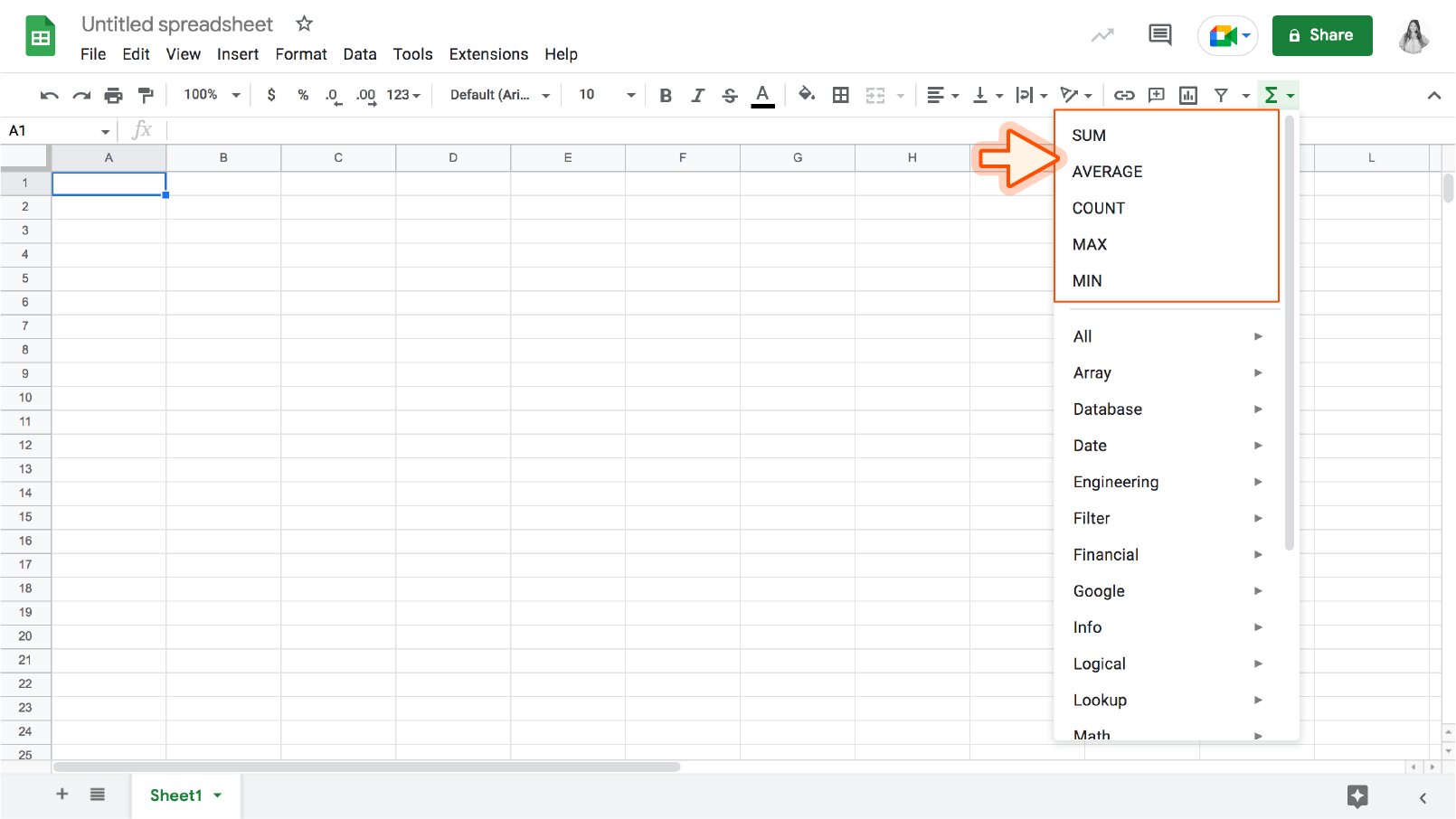
Google Sheets provides several functions and tools that make it easy to round numbers according to your specific requirements. Whether you need to round to a specific decimal place, round to the nearest 10, 100, or 1000, or round to significant figures, Google Sheets has got you covered.
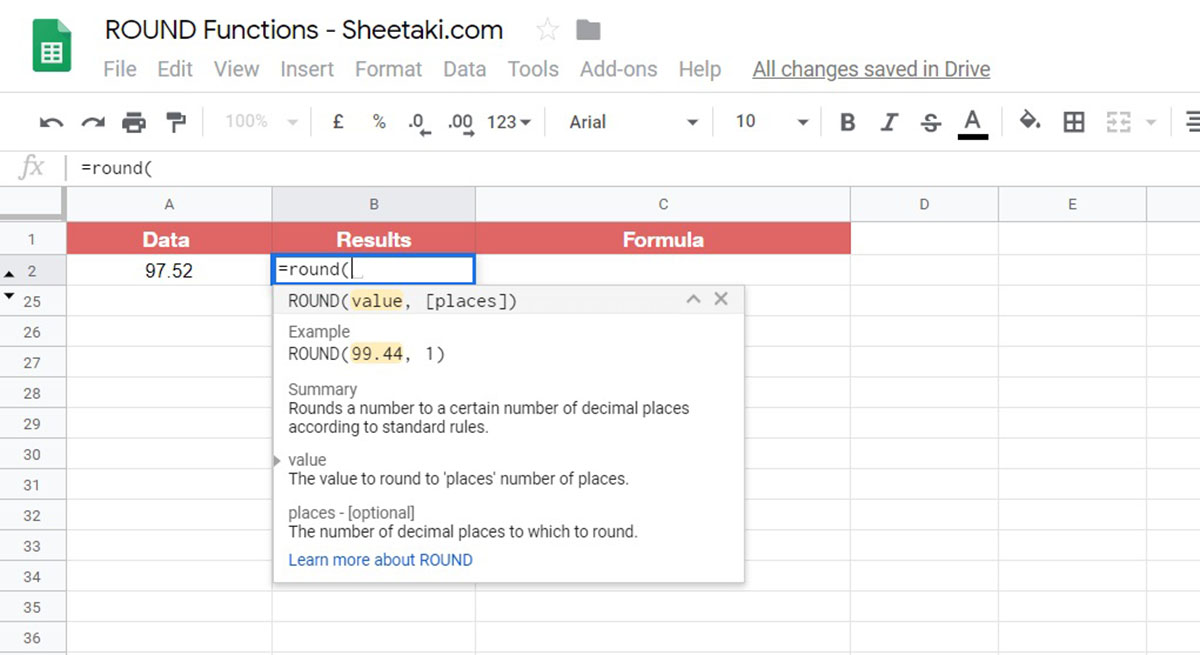
To begin rounding numbers in Google Sheets, you can use the ROUND function. This function allows you to specify the number you want to round and the number of decimal places to round to. For example, if you have a number in cell A1 and you want to round it to two decimal places, you can use the formula: =ROUND(A1, 2).
Additionally, if you want to round a number to the nearest whole number, you can use the ROUNDUP or ROUNDDOWN functions. The ROUNDUP function rounds up to the nearest whole number, while the ROUNDDOWN function rounds down to the nearest whole number. For example, to round the number in cell A1 to the nearest whole number, you can use the formula: =ROUNDUP(A1, 0) or =ROUNDDOWN(A1, 0).
If you need to round a number to the nearest 10, 100, or 1000, Google Sheets offers the MROUND function. This function allows you to specify the number you want to round and the multiple to round to. For instance, if you have a number in cell A1 and you want to round it to the nearest 10, you can use the formula: =MROUND(A1,10).
When it comes to rounding numbers to significant figures, you can use the ROUND function in combination with the POWER function. The POWER function helps determine the power of 10 to use for rounding. For example, if you have a number in cell A1 and you want to round it to 3 significant figures, you can use the formula: =ROUND(A1, -POWER(10, -2)).
In summary, Google Sheets offers a range of functions and tools that allow you to round numbers to meet your specific needs and preferences. Whether it’s rounding to a specific decimal place, rounding to the nearest 10, 100, or 1000, rounding to significant figures, or rounding up or down, you can easily manipulate your data to present it in a cleaner and more organized format.
Rounding to a Specific Decimal Place
Rounding numbers to a specific decimal place is a common requirement when working with financial data, measurements, or any situation where precision is crucial. Fortunately, Google Sheets provides a simple and effective way to round numbers to the desired decimal place.
To round a number to a specific decimal place in Google Sheets, you can use the ROUND function. The ROUND function accepts two arguments: the number you want to round and the number of decimal places to round to.
For example, let’s say you have a number in cell A1 and you want to round it to 2 decimal places. You can use the formula: =ROUND(A1, 2). This formula will round the number in cell A1 to the nearest 2 decimal places.
If you want to round up or down to a specific decimal place, you can use the ROUNDUP or ROUNDDOWN function instead. The ROUNDUP function rounds the number up to the specified decimal place, while the ROUNDDOWN function rounds the number down.
For instance, if you have a number in cell A1 and you want to round it up to 3 decimal places, you can use the formula: =ROUNDUP(A1, 3). This will round the number in cell A1 up to the nearest 3 decimal places.
On the other hand, if you want to round the number down to 4 decimal places, you can use the formula: =ROUNDDOWN(A1, 4). This will round the number in cell A1 down to the nearest 4 decimal places.
By using the ROUND, ROUNDUP, or ROUNDDOWN functions with the appropriate decimal places, you can easily round numbers in Google Sheets to meet your specific requirements. This feature is particularly useful when dealing with financial calculations, scientific measurements, or any situation where precision matters.
Rounding to the Nearest 10, 100, or 1000
In some cases, you may want to round numbers to the nearest 10, 100, or 1000 for better readability or when dealing with large quantities. Google Sheets provides a convenient function called MROUND to achieve this.
To round a number to the nearest multiple of 10, you can use the MROUND function. The MROUND function accepts two arguments: the number you want to round and the multiple to round to.
For example, suppose you have a number in cell A1 and you want to round it to the nearest multiple of 10. You can use the formula: =MROUND(A1, 10). This formula will round the number in cell A1 to the nearest multiple of 10.
If you want to round to the nearest multiple of 100, you can modify the formula to: =MROUND(A1, 100). This will round the number in cell A1 to the nearest multiple of 100.
Similarly, if you need to round to the nearest multiple of 1000, you can use the formula: =MROUND(A1, 1000). This will round the number in cell A1 to the nearest multiple of 1000.
The MROUND function is particularly useful when dealing with large numbers or when you want to simplify the representation of your data. It helps create more understandable and aesthetically pleasing reports or presentations.
By utilizing the MROUND function with the appropriate multiple, you can easily round numbers to the nearest 10, 100, or 1000 in Google Sheets. This feature is especially beneficial when working with quantities, measurements, or any situation where rounding to a specific magnitude is desired.
Rounding to Significant Figures
Rounding to significant figures is a common practice in scientific and technical fields where accuracy and precision are paramount. It helps to ensure the appropriate level of detail without misleading or overstating the significance of the data. In Google Sheets, you can easily round numbers to significant figures using a combination of the ROUND and POWER functions.
To round a number to the desired significant figures, you need to determine the power of 10 to use for rounding. The power of 10 is calculated using the POWER function, which takes two arguments: the base (10) and the exponent. The exponent is the negative of the desired number of significant figures. For example, if you want to round to 3 significant figures, the exponent will be -3.
Once you have the power of 10, you can use the ROUND function in combination with the POWER function to round the number. The ROUND function rounds the number to the specified number of digits based on the power of 10.
For example, let’s say you have a number in cell A1 and you want to round it to 3 significant figures. You can use the formula: =ROUND(A1, -POWER(10, -3)). The POWER function calculates the power of 10 (-3 in this case), and then the ROUND function rounds the number in cell A1 to 3 significant figures based on that power of 10.
By adjusting the exponent in the formula, you can easily round numbers to any desired number of significant figures. This allows you to present your data accurately and precisely, without unnecessary digits or loss of important information.
Rounding to significant figures is particularly useful when dealing with scientific measurements, data analysis, or any situation where maintaining precision is crucial. It ensures that your numbers are rounded appropriately, taking into account the significance of the digits.
In summary, Google Sheets provides a straightforward method to round numbers to significant figures. By combining the ROUND and POWER functions, you can accurately round numbers to the desired level of precision, making your data more meaningful and reliable.
Rounding Up or Down
Sometimes, rounding a number to the nearest whole number may not be enough. You may need to round a number up or down based on specific criteria, such as rounding up to the nearest integer or rounding down to the nearest multiple of 10. In Google Sheets, there are functions available to help you achieve this.
To round a number up to the nearest whole number, you can use the ROUNDUP function. The ROUNDUP function takes two arguments: the number you want to round and the number of decimal places to round up to. For example, if you have a number in cell A1 and you want to round it up to the nearest whole number, you can use the formula: =ROUNDUP(A1, 0). This formula will round the number in cell A1 up to the nearest whole number.
On the other hand, if you want to round a number down to the nearest whole number, you can use the ROUNDDOWN function. The ROUNDDOWN function also takes two arguments: the number you want to round and the number of decimal places to round down to. For example, to round the number in cell A1 down to the nearest whole number, you can use the formula: =ROUNDDOWN(A1, 0).
In addition to rounding up or down to the nearest whole number, you can also round up or down to multiples of a specific value. For example, if you want to round a number up to the nearest multiple of 10, you can use the CEILING function. The CEILING function accepts two arguments: the number you want to round and the multiple to round up to.
For instance, suppose you have a number in cell A1 and you want to round it up to the nearest multiple of 10. You can use the formula: =CEILING(A1, 10). This will round the number in cell A1 up to the nearest multiple of 10.
Similarly, if you want to round a number down to the nearest multiple of 10, you can use the FLOOR function. The FLOOR function takes two arguments: the number you want to round and the multiple to round down to. For example, to round the number in cell A1 down to the nearest multiple of 10, you can use the formula: =FLOOR(A1, 10).
By utilizing the ROUNDUP, ROUNDDOWN, CEILING, and FLOOR functions with the desired arguments, you can easily round numbers up or down based on specific criteria. These functions offer flexibility and precision, allowing you to fine-tune the rounding behavior to meet your unique requirements.
Rounding Formulas in Google Sheets
Google Sheets provides a variety of rounding formulas that offer a higher level of flexibility and customization when rounding numbers. These formulas allow you to apply rounding to specific cells, ranges, or even entire arrays of data.
One commonly used rounding formula is the ROUND function. This function can be used to round numbers to a specified number of decimal places. For example, if you have a range of numbers in cells A1 to A10 and you want to round them to 2 decimal places, you can use the formula: =ROUND(A1:A10, 2). This formula will round all the numbers in the specified range to 2 decimal places.
If you prefer to round numbers up to the nearest whole number, you can use the CEILING function. Similar to the ROUND function, the CEILING function can be applied to a range of cells. For example, to round up all the numbers in cells A1 to A10 to the nearest whole number, you can use the formula: =CEILING(A1:A10, 1).
Alternatively, if you want to round numbers down to the nearest whole number, you can use the FLOOR function. The FLOOR function works similarly to the CEILING function but rounds numbers down instead. For example, to round down all the numbers in cells A1 to A10 to the nearest whole number, you can use the formula: =FLOOR(A1:A10, 1).
In addition to the ROUND, CEILING, and FLOOR functions, Google Sheets also provides the INT function, which rounds numbers down to the nearest integer. This function is particularly useful when working with whole numbers. For example, if you have a range of numbers in cells A1 to A10 and you want to round them down to the nearest integer, you can use the formula: =INT(A1:A10).
By utilizing these rounding formulas in Google Sheets, you can easily apply rounding to specific cells, ranges, or arrays of data. These formulas allow for greater precision and control when working with numbers, ensuring that your data is rounded according to your desired criteria.
Rounding Numbers in Arrays
Google Sheets allows you to work with arrays of data, making it easy to perform calculations and manipulations on multiple numbers simultaneously. When it comes to rounding numbers in arrays, there are various methods you can use to ensure consistency and efficiency.
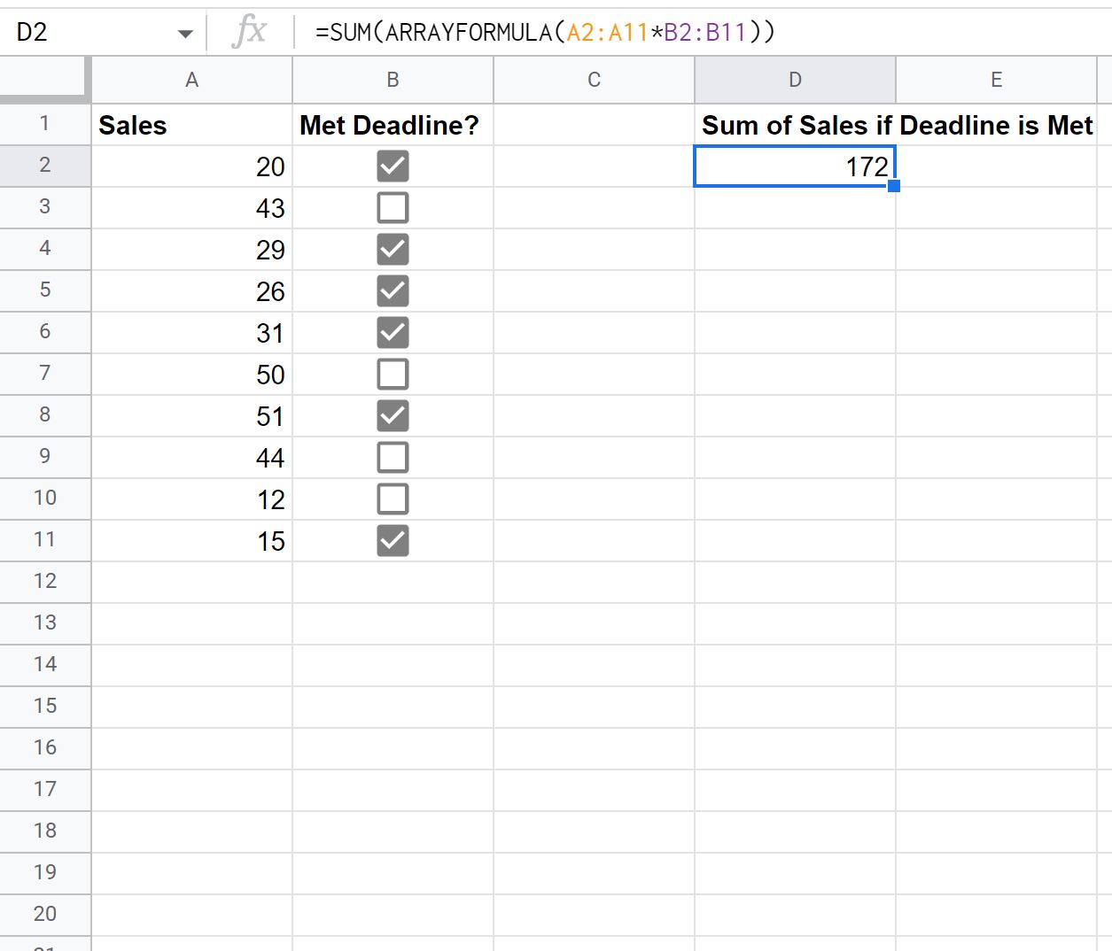
One way to round numbers in arrays is by using the ARRAYFORMULA function in combination with the desired rounding formula. For example, if you have a range of numbers in cells A1 to A10 and you want to round them to 2 decimal places, you can use the formula: =ARRAYFORMULA(ROUND(A1:A10, 2)). This formula will apply the ROUND function to each element in the array and round them to 2 decimal places.
In addition to the ARRAYFORMULA function, you can also use the ROUNDUP, ROUNDDOWN, CEILING, or FLOOR functions in combination with the ARRAYFORMULA function to round numbers in arrays. This allows you to round up, round down, round to the nearest multiple, or round to the nearest whole number in an array of data.
For example, suppose you have a range of numbers in cells A1 to A10 and you want to round them up to the nearest whole number. You can use the formula: =ARRAYFORMULA(ROUNDUP(A1:A10, 0)). This formula will round up each number in the array to the nearest whole number.
Similarly, if you want to round the numbers in an array down to the nearest multiple of 10, you can use the formula: =ARRAYFORMULA(FLOOR(A1:A10, 10)). This formula will round down each number in the array to the nearest multiple of 10.
By leveraging the ARRAYFORMULA function along with the appropriate rounding formula, you can efficiently round numbers in arrays and apply the desired rounding behavior to multiple data points simultaneously. This saves time and ensures consistency in your calculations.
Whether you need to round numbers in a small array or a large dataset, Google Sheets provides the flexibility and functionality to handle arrays of data effectively. These techniques allow you to manipulate and round numbers in arrays with ease, helping you streamline your data analysis and calculations.
Applying Rounding to Multiple Cells
In Google Sheets, you can easily apply rounding to multiple cells by using simple formulas and techniques. Whether you want to round numbers in a specific range or across an entire column or row, there are several methods available to accomplish this.
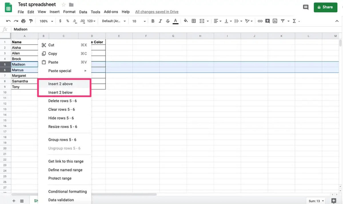
One way to apply rounding to multiple cells is by using the Fill Handle feature in Google Sheets. Simply enter the rounding formula in the first cell, then click and drag the fill handle (located in the bottom right corner of the cell) down or across the range of cells you want to apply the rounding to. Google Sheets will automatically adjust the cell references in the formula as you drag the fill handle, allowing you to quickly and efficiently apply the rounding formula to multiple cells.
Another method is to use the ARRAYFORMULA function. This function allows you to perform calculations on an entire range of cells at once. To apply rounding to multiple cells using ARRAYFORMULA, enter the rounding formula in the first cell of the target range and wrap it within the ARRAYFORMULA function. For example, if you want to round all the numbers in column A to 2 decimal places, you can use the formula: =ARRAYFORMULA(ROUND(A:A, 2)). This formula will apply the rounding function to every cell in column A, rounding each number to 2 decimal places.
If you have specific criteria for rounding multiple cells, you can combine the rounding formula with an IF statement. The IF statement allows you to add conditions that must be met for the rounding to occur. For example, if you want to round numbers in column A only if they are greater than 10, you can use the formula: =ARRAYFORMULA(IF(A:A>10, ROUND(A:A, 0), A:A)). This formula will round the numbers in column A to the nearest whole number if they are greater than 10, and leave them unchanged otherwise.
By utilizing the Fill Handle, ARRAYFORMULA, and IF statement in Google Sheets, you can easily apply rounding to multiple cells. These techniques help streamline your workflow and save time when working with large datasets or when you need to round a significant number of values.
Examples of Rounding Numbers in Google Sheets
Let’s dive into some practical examples of how to round numbers in Google Sheets using various rounding techniques. These examples will help illustrate how to apply rounding formulas to different scenarios, allowing you to adapt them to your specific needs.
Example 1: Rounding to 2 Decimal Places:
If you have a range of numbers in cells A1 to A10 and you want to round them to 2 decimal places, you can use the formula: =ROUND(A1:A10, 2). This will round each number in the range to the nearest 2 decimal places.
Example 2: Rounding Up to the Nearest Whole Number:
Suppose you have a range of numbers in cells B1 to B10 and you want to round them up to the nearest whole number. You can use the formula: =ROUNDUP(B1:B10, 0). This will round up each number in the range to the nearest whole number.
Example 3: Rounding Down to the Nearest Multiple:
Let’s say you have a range of numbers in cells C1 to C10 and you want to round them down to the nearest multiple of 5. You can use the formula: =FLOOR(C1:C10, 5). This will round down each number in the range to the nearest multiple of 5.
Example 4: Rounding to Significant Figures:
Suppose you have a range of numbers in cells D1 to D10 and you want to round them to 3 significant figures. You can use the formula: =ROUND(D1:D10, -POWER(10, -3)). This will round each number in the range to 3 significant figures.
Example 5: Rounding with Condition using IF statement:
If you have a range of numbers in cells E1 to E10 and you only want to round numbers that are greater than 50, you can use the formula: =ARRAYFORMULA(IF(E1:E10>50, ROUND(E1:E10, -1), E1:E10)). This formula will round the numbers greater than 50 to the nearest 10, and leave the rest of the numbers unchanged.
These examples showcase just a few of the many possibilities for rounding numbers in Google Sheets. By leveraging these techniques and formulas, you can easily customize your rounding to suit your specific requirements and achieve the desired level of precision and accuracy.
Conclusion
Rounding numbers in Google Sheets is a fundamental skill that can greatly enhance the presentation, accuracy, and readability of your data. Whether you need to round to a specific decimal place, round to the nearest 10, 100, or 1000, round to significant figures, or round up or down based on specific criteria, Google Sheets provides a range of functions and tools to meet your needs.
By using formulas such as ROUND, ROUNDUP, ROUNDDOWN, CEILING, FLOOR, and ARRAYFORMULA, you can easily apply rounding to individual cells, ranges, arrays, or entire columns in your spreadsheet. These tools allow for precise calculations and manipulation of numbers, ensuring that your data is presented in the desired format.
From financial reports to scientific measurements, rounding numbers is a common practice in various fields. Rounding not only simplifies complex data but also improves its interpretability. Whether you are a student, professional, or business owner, mastering the art of rounding numbers in Google Sheets can help you create cleaner, more organized, and visually appealing spreadsheets.
Remember, it is important to strike a balance between precision and readability when it comes to rounding numbers. Consider the context of your data and the level of accuracy required for your particular task. By understanding the available rounding techniques and selecting the appropriate method for your needs, you can ensure that your rounded numbers accurately represent the underlying data.
So, explore the rounding functions, formulas, and techniques discussed in this guide, experiment with different scenarios, and incorporate them into your Google Sheets workflow. By doing so, you can improve the quality, clarity, and professionalism of your spreadsheets, making your data more meaningful and impactful.