How To Calculate Average On Google Sheets

Introduction

Welcome to our guide on how to calculate averages using Google Sheets! Averages are fundamental statistical measures that allow us to understand the central tendency of a set of values. Whether you’re a student, a data analyst, or simply someone who needs to calculate the average of a series of numbers, Google Sheets provides a powerful and intuitive platform to perform these calculations.

In this article, we will walk you through the step-by-step process of calculating averages in Google Sheets. We will cover the basics of understanding what averages are and how they are calculated, as well as more advanced techniques like calculating weighted averages. We will also explore various customization options and strategies to deal with empty cells or errors that may be present in your data.

But first, let’s take a moment to understand the importance of averages. Averages provide us with a single representative value that summarizes a given dataset. They help us make sense of large amounts of data by distilling it down to a single number that reflects its central tendency. Averages are widely used in a variety of fields, including education, finance, and business, to gain insights and make informed decisions based on the data available.

Google Sheets is a powerful cloud-based spreadsheet software that allows users to perform complex calculations, visualize data, and collaborate with others in real-time. It offers a simple and user-friendly interface, making it accessible to beginners while providing advanced features for more experienced users.

Throughout this guide, we will explore the various tools and functions provided by Google Sheets to help you calculate averages efficiently and effectively. So, whether you’re a novice or an experienced user, let’s dive into the world of calculating averages on Google Sheets and unlock the potential of your data!

Understanding Averages

Averages are statistical measures that provide insight into the central tendency of a set of values. They are commonly used to summarize data and gain a better understanding of the overall picture. There are different types of averages, but the most commonly used one is the arithmetic mean.

The arithmetic mean is calculated by summing up all the values in a dataset and dividing the total by the number of values. This provides a single representative value that reflects the average of the entire dataset. It is straightforward to compute and provides a useful summary of the data.

However, it is important to note that averages can be affected by extreme values, known as outliers. These outliers can skew the average and may not accurately represent the majority of the data. Therefore, it’s important to consider the context and characteristics of the dataset when interpreting the average.

Another type of average is the weighted average. Unlike the arithmetic mean, the weighted average assigns different weights to each value in the dataset based on their importance or significance. This type of average is commonly used when different values have different levels of relevance or importance within the dataset.

Understanding how to calculate and interpret averages is essential in various fields. In finance, averages are used to analyze stock market trends and assess investment performance. In education, averages are used to evaluate student performance and grade assignments. In business, averages help analyze sales data and track performance indicators.

Having a solid understanding of averages will allow you to make informed decisions based on data. In the next sections, we will explore how to use Google Sheets to calculate averages efficiently and effectively. We will cover basic techniques as well as more advanced scenarios, so you’re fully equipped to handle any averaging task.

Creating a Spreadsheet on Google Sheets

Before we start calculating averages on Google Sheets, we need to create a spreadsheet to work with. Google Sheets provides a user-friendly interface for creating and organizing data in a tabular format. Here’s how you can create a spreadsheet:

1. Open Google Sheets by going to https://docs.google.com/spreadsheets and signing into your Google account.
2. Once you’re on the Google Sheets homepage, click on the “Blank” option to create a new spreadsheet from scratch.
3. The new spreadsheet will open with a blank grid of rows and columns.
4. You can customize the spreadsheet by giving it a meaningful name by clicking on the “Untitled spreadsheet” title at the top and entering a new name.
5. To organize your data, you can create multiple sheets within the same spreadsheet. This can be done by clicking on the “+” button at the bottom left corner of the screen. Each sheet can contain different sets of data or serve different purposes.
6. Customize the formatting of your spreadsheet by selecting the desired font, size, and color options from the toolbar at the top. You can also adjust the width and height of rows and columns to accommodate your data.
7. Now that you have created your spreadsheet, you can start entering your data and perform calculations, including calculating averages.

Creating a spreadsheet on Google Sheets is quick and easy. It provides you with a versatile workspace to input and analyze your data. You can access your spreadsheet from any device with an internet connection, making it convenient for collaboration and remote work.

Now that you have your spreadsheet ready, let’s move on to the next section, where we’ll dive into entering data into the spreadsheet and learn how to calculate averages in Google Sheets.

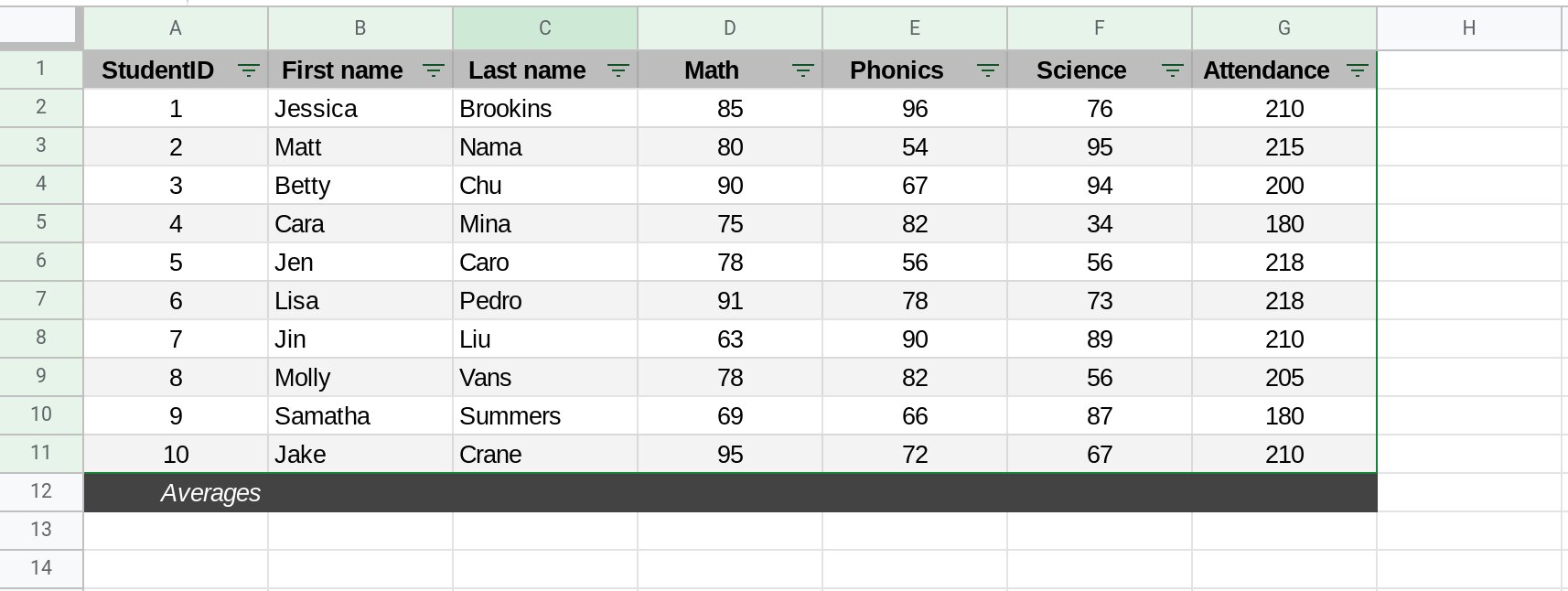
Entering Data into the Spreadsheet

Now that you have created your spreadsheet on Google Sheets, it’s time to enter your data. The data you input will form the basis for calculating averages and performing other calculations. Here’s how you can enter data into your spreadsheet:

1. Select the cell where you want to enter your data. You can do this by clicking on the desired cell or by using the arrow keys to navigate to the cell.
2. Type in the data value you want to enter. For example, if you’re entering a series of numbers, simply type each number into the corresponding cell. You can also enter text, dates, and other types of data.
3. Press Enter or use the Tab key to move to the next cell in the row. If you want to move to the cell below, press the Enter key again.
4. Continue entering your data into the cells, moving from left to right or top to bottom, depending on your preference.
5. If you want to edit or modify a cell’s content, simply double-click on the cell and make the necessary changes.
6. You can use the mouse to drag and select multiple cells to enter data in bulk. This is useful when you have a large dataset to input.
7. To delete a value from a cell, select the cell and press the Delete or Backspace key on your keyboard.

It’s worth mentioning that you can format cells to reflect the data type you’re entering. For example, you can format a cell as a number, currency, date, or percentage. This can be done by selecting the cell or cells, right-clicking, and choosing the “Format” option from the context menu.

By entering your data accurately and organizing it effectively in your spreadsheet, you’ll ensure that your calculations, including the calculation of averages, are performed correctly. In the next section, we’ll explore how to use Google Sheets’ built-in functions to calculate averages easily.

Using the AVERAGE Function

Google Sheets provides a built-in function called AVERAGE for calculating the average of a set of values. This function automates the manual calculation process and makes it quick and easy to obtain accurate averages. Here’s how you can use the AVERAGE function:

1. Select the cell where you want the average to appear.
2. Type =AVERAGE(
3. Select the range of cells that contain the values you want to average. For example, to average the numbers in cells A1 to A10, you would select A1:A10.
4. Type the closing parenthesis ) and press Enter.

The AVERAGE function will calculate and display the average of the selected range of cells. The resulting average will automatically update if the values in the range change.

For example, if you have a set of numbers in cells A1 to A10 and you want to calculate their average, you would enter =AVERAGE(A1:A10) in a different cell. The calculated average will be displayed in that cell.

It’s important to note that the AVERAGE function only considers numeric values in the selected range. Any text or empty cells will be ignored in the calculation. This allows you to exclude non-numeric data from skewing the average.

You can also use the AVERAGE function to calculate averages across multiple columns or rows. Simply select the desired range of cells that span across the columns or rows you want to include in the calculation. For example, to calculate the average of multiple columns A, B, and C, you would select the range A1:C10.

Now that you know how to use the AVERAGE function, you can easily calculate averages in Google Sheets. In the next section, we’ll explore how to calculate the average of a range of cells using a slightly different approach.

Calculating the Average of a Range of Cells

In addition to using the AVERAGE function, Google Sheets provides another method to calculate the average of a range of cells. This approach involves manually summing up the values in the range and dividing the total by the number of cells. Here’s how you can calculate the average of a range of cells:

1. Select the cell where you want the average to appear.
2. Type =SUM(
3. Select the range of cells that you want to include in the average calculation. For example, to average the numbers in cells A1 to A10, you would select A1:A10.
4. Type )/COUNT(
5. Select the same range of cells as in step 3.
6. Type ) and press Enter.

The formula will calculate the sum of the values in the selected range and divide it by the count of cells in that range. This will give you the average of the range.

For example, if you want to calculate the average of the range A1 to A10, you would enter =(SUM(A1:A10))/COUNT(A1:A10) in a different cell. The calculated average will be displayed in that cell.

Using this method allows you to have more flexibility and control over the calculation logic. For instance, you may want to exclude certain cells from the average calculation by selecting a specific range or specify different ranges for the sum and count functions.

This approach is especially useful when you need to calculate additional statistics, such as the sum or count, alongside the average. By using the combination of the SUM and COUNT functions, you can obtain more comprehensive insights about your data.

Now that you understand how to calculate the average of a range of cells using this method, you have multiple options to calculate averages in Google Sheets. In the next section, we will explore how to calculate weighted averages for scenarios where different values carry different weights.

Calculating Weighted Averages

In some situations, you may need to calculate a weighted average where different values in your dataset carry different weights or importance. A weighted average takes into account these varying weights to provide a more accurate representation of the data. Google Sheets offers a simple way to calculate weighted averages using the SUMPRODUCT function. Here’s how:

1. Select the cell where you want the weighted average to appear.
2. Type =SUMPRODUCT(
3. Select the range of cells that contain the values you want to average.
4. Type ,
5. Select the range of cells that contain the corresponding weights for each value in the previous range.
6. Type )/SUM(
7. Select the range of cells that contain the weights.
8. Type ) and press Enter.

The formula will multiply each value in the first range by its corresponding weight and then sum up the products. This sum is then divided by the sum of the weights to calculate the weighted average.

For example, if you have a set of numbers in cells A1 to A10 and their corresponding weights in cells B1 to B10, you would enter =SUMPRODUCT(A1:A10, B1:B10)/SUM(B1:B10) in a different cell. The calculated weighted average will be displayed in that cell.

Weighted averages are commonly used in various scenarios, such as calculating weighted GPA in education, analyzing financial portfolios based on asset weights, or determining performance ratings based on different criteria. By incorporating weights into your average calculations, you can obtain more accurate and meaningful results.

Now that you know how to calculate weighted averages in Google Sheets, you have the tools to handle scenarios where different values have varying levels of significance. In the next section, we’ll explore how you can customize averaging parameters to suit your specific needs.

Customizing Averaging Parameters

Google Sheets provides flexibility in customizing averaging parameters to fit your specific needs. By adjusting these parameters, you can modify the way averages are calculated, consider specific criteria, or exclude certain values from the calculations. Here are some ways you can customize averaging parameters:

• Exclude certain values: If you want to exclude specific values from the average calculation, you can use the AVERAGEIF or AVERAGEIFS functions. These functions allow you to specify criteria for inclusion or exclusion. For example, you can calculate the average of values in a range that meet a certain condition, such as greater than a particular threshold.
• Round decimals: By default, Google Sheets displays the average with a certain number of decimal places. However, you can customize the number of decimal places displayed by using the ROUND function. This allows you to round the average to the desired precision.
• Adjust weightings: When calculating weighted averages, you can modify the weights assigned to each value to emphasize or de-emphasize their impact on the overall average. This can be done by changing the weight values in the range of cells used for calculating the weighted average.
• Use alternative averaging methods: Apart from the arithmetic mean, Google Sheets provides other averaging functions, such as MEDIAN, MODE, and GEOMEAN. These functions offer alternative ways to calculate averages based on specific characteristics of the dataset.

Customizing averaging parameters allows you to fine-tune your calculations to meet your specific requirements. By leveraging these customization options, you can gain more control over your data analysis and ensure that the calculated averages align with your intended interpretations.

Experimenting with different parameters and functions in Google Sheets will enable you to explore various approaches and adapt them according to the nature of your data and the insights you’re seeking.

Now that you have an understanding of how to customize averaging parameters, you can tailor your average calculations to suit your unique needs. In the next section, we’ll delve into strategies for dealing with empty cells or errors that may be present in your dataset.

Dealing with Empty Cells or Errors

When working with data in Google Sheets, it’s common to encounter empty cells or errors, such as #DIV/0! or #VALUE!. These can affect the accuracy of your average calculations if not handled properly. Here are some strategies for dealing with empty cells or errors in your dataset:

• Ignoring empty cells: If your dataset contains empty cells, you can choose to exclude them from the average calculation. When using the AVERAGE or AVERAGEIF functions, Google Sheets automatically ignores empty cells, resulting in the average being calculated based only on non-empty cells. This ensures that empty cells do not distort the average.
• Handling errors: When errors occur in your data, it’s important to address them appropriately. For example, if you encounter a #DIV/0! error, it means that you’re trying to divide by zero in a calculation. You can use the IFERROR function to replace the error with a specific value or a blank cell. This allows you to perform calculations without the risk of errors impeding your average calculations.
• Filtering out errors: If you want to exclude cells with specific errors from your average calculation, you can use the AVERAGEIF or AVERAGEIFS functions in combination with the ISERROR or ISERR functions. This allows you to set criteria that exclude cells with errors, ensuring that only valid values contribute to the average calculation.
• Replacing errors: Alternatively, you may choose to replace errors with a specific value before calculating the average. This can be done using the IF function in combination with the ISERROR or ISERR function. By replacing errors with a designated value, you can include them in the average calculation while minimizing their impact on the overall result.

By employing these strategies, you can effectively handle empty cells or errors in your dataset, ensuring that your average calculations are accurate and reliable. It’s crucial to consider these scenarios and adopt the appropriate approach based on your specific data and objectives.

Now that you have techniques for dealing with empty cells or errors, you are better equipped to address data discrepancies and perform accurate average calculations. In the next section, we’ll explore how you can apply averages to multiple columns or rows for a more comprehensive analysis.

Applying Averages to Multiple Columns or Rows

In many cases, you may need to calculate averages across multiple columns or rows to gain a broader perspective or compare different sets of data. Google Sheets provides a convenient way to apply averages to multiple columns or rows using built-in functions. Here’s how you can do it:

• Averaging multiple columns: To calculate the average of values in multiple columns, you can use the AVERAGE function in combination with the colon (:) operator. For example, if you have values in columns A, B, and C, you can enter =AVERAGE(A:C) in a different cell to obtain the average of all the values in those columns. This approach allows you to calculate the overall average across multiple related data sets.
• Averaging multiple rows: Similarly, to calculate the average of values in multiple rows, you can use the AVERAGE function with the row number ranges. For example, if you have values in rows 1 to 5, you can enter =AVERAGE(1:5) in a cell to calculate the average of all the values in those rows. This allows you to calculate an overall average across different data sets within the same column.
• Averaging multiple columns or rows selectively: If you want to calculate averages across specific columns or rows rather than the entire range, you can manually select the desired cells or ranges for the average calculation. You can leverage the AVERAGE or AVERAGEIF functions to specify criteria and include or exclude certain cells in the calculation.

Applying averages to multiple columns or rows allows you to analyze and compare data sets comprehensively. It enables you to identify trends, patterns, or differences across different dimensions of your data, providing deeper insights into your analysis.

By utilizing these techniques in Google Sheets, you can easily calculate averages across various columns or rows without the need for complex manual calculations. This saves time and ensures accuracy in your data analysis.

Now that you know how to apply averages to multiple columns or rows in Google Sheets, you have the flexibility to explore and analyze different dimensions of your data. In the next section, we’ll explore how you can visualize averages using charts and graphs to enhance your data presentation.

Using Filters with Averages

In Google Sheets, filters allow you to display specific subsets of data, making it easier to analyze and calculate averages for specific criteria. By applying filters to your data, you can refine your average calculations and gain more targeted insights. Here’s how you can use filters with averages:

• Filtering by value: You can use filters to select specific values in a column and calculate the average based on that subset of data. To do this, select the column you want to filter, go to the Data menu, and choose “Create a filter.” Then, use the filter dropdown to select the desired values. The average will update based on the filtered data.
• Filtering by condition: In addition to filtering by value, you can apply filters based on conditions. For example, you can filter based on values that are greater than a certain threshold, equal to a specific value, or within a certain range. By specifying the condition in the filter, you can calculate the average based on the filtered data that meets that particular criterion.
• Multiple filters: You can also combine multiple filters to further refine your average calculations. By applying multiple filters based on different criteria, you can narrow down your dataset to a specific subset and calculate averages that are relevant to your analysis. This allows for granular control over the data included in the average calculation.

Using filters with averages provides a powerful way to focus on specific subsets of data and generate more meaningful insights. Filters allow you to segment your data based on specific criteria, making it easier to identify patterns, trends, or outliers within particular data subsets.

By harnessing the filtering capabilities of Google Sheets, you can perform average calculations on subsets of data that are more relevant to your analysis, providing a more accurate representation of the desired metrics.

Now that you understand how to use filters with averages in Google Sheets, you can apply these techniques to make more targeted calculations and gain deeper insights into your data. In the next section, we’ll explore how you can visualize averages using charts and graphs to enhance the presentation of your data.

Visualizing Averages with Charts and Graphs

Visualizing averages using charts and graphs is an effective way to present and understand data trends at a glance. Google Sheets offers a range of intuitive tools that allow you to create visually appealing charts based on your calculated averages. Here’s how you can visualize averages with charts and graphs:

1. Select the range of data that includes the average values you want to visualize, along with any corresponding labels or categories.
2. Go to the Insert menu and choose the type of chart or graph that best represents your data and analysis. Common chart types for visualizing averages include bar charts, line charts, column charts, and pie charts.
3. Customize the chart as needed by adjusting various settings, such as the colors, titles, axes labels, or data ranges. This allows you to highlight the averages and provide additional context to aid interpretation.
4. Add data labels or tooltips to the chart to display specific average values or relevant information when a data point is hovered over or clicked on.
5. Choose an appropriate chart layout, such as stacking columns or lines, to showcase multiple averages side by side or over time.
6. Consider exploring different types of charts or combinations of charts to create more complex visualizations. This can include using dual-axis charts to show averages alongside other metrics or utilizing combination charts to display multiple average calculations simultaneously.

Visualizing averages with charts and graphs enables you to communicate key insights and patterns effectively. The visual representation helps your audience comprehend the data more readily, grasp trends, and make comparisons. It can also aid in spotting outliers or anomalies within the dataset.

With Google Sheets’ charting capabilities, you can easily create dynamic, interactive, and visually appealing charts to showcase your average calculations. These charts can be easily updated as your data changes, ensuring that your visualizations stay current and reflect the most recent averages.

Now that you know how to visualize averages with charts and graphs in Google Sheets, you have a powerful tool to present your average calculations and enhance the communicative impact of your data. In the next section, we’ll recap the key points and provide some final tips for working with averages in Google Sheets.

Summary and Final Tips

Calculating averages in Google Sheets is a valuable skill that allows you to gain insights and make informed decisions based on your data. Here’s a summary of the key points discussed in this guide:

• Averages provide a measure of central tendency and are commonly used to summarize data.
• Google Sheets offers built-in functions like AVERAGE and SUMPRODUCT for calculating averages and weighted averages.
• Customizing averaging parameters allows you to exclude empty cells, handle errors, and modify weights to suit your specific needs.
• Applying averages to multiple columns or rows allows for comprehensive analysis and comparison of data sets.
• Using filters with averages lets you focus on specific subsets of data and refine your calculations.
• Visualizing averages with charts and graphs enhances data presentation and aids in understanding trends.

As you work with averages in Google Sheets, keep the following tips in mind:

• Ensure the accuracy of your data entry to obtain reliable average calculations.
• Be mindful of empty cells or errors and handle them appropriately to avoid distorting averages.
• Experiment with different functions, filters, and customizations to tailor your average calculations to your specific needs.
• Consider visualizing your averages using charts and graphs to enhance data presentation and facilitate interpretation.
• Regularly validate and update your averages as your data changes to maintain accuracy in your analysis.

By following these tips and utilizing the features and functions available in Google Sheets, you can confidently calculate and work with averages, empowering you to gain valuable insights from your data.

Now that you have a comprehensive understanding of how to calculate averages in Google Sheets, you’re ready to apply these techniques to your own data analysis tasks. Explore the various tools and functions available and unlock the full potential of your data!