Introduction
Welcome to the world of Google Sheets! Whether you are a professional or a student, Google Sheets can be an incredibly powerful tool for organizing and analyzing data. With its comprehensive set of functions and features, it provides a convenient and efficient way to work with data in a spreadsheet format.
In this article, we will explore the basics of Google Sheets and delve into some advanced functions that can take your data manipulation and analysis skills to the next level. Whether you are a beginner or an experienced user, this guide will help you navigate through the intricacies of Google Sheets.
Google Sheets is a cloud-based spreadsheet software that allows you to create, edit, and share spreadsheets online. It offers a wide range of functions that can be used to perform calculations, create formulas, and manipulate data. Whether you need to perform simple calculations like summing up a column of numbers or complex tasks like using conditional statements to filter and analyze data, Google Sheets has got you covered.
One of the advantages of Google Sheets is its collaborative features. Multiple people can work on the same spreadsheet simultaneously, making it an excellent tool for teamwork and collaboration. Additionally, Google Sheets automatically saves your work as you go, eliminating the risk of losing important data.
Another great feature of Google Sheets is its integration with other Google services, such as Google Drive and Google Forms. You can easily import and export data from various sources, collaborate with teammates, and share your spreadsheets with others.
Although Google Sheets may seem overwhelming at first, don’t worry! We will guide you through the basic functions, such as summing, averaging, and counting values, as well as the more advanced functions, such as the powerful IF and VLOOKUP functions. We will also share some tips and tricks to enhance your productivity and make your spreadsheet work more efficient and effective.
Now, without further ado, let’s dive into the world of Google Sheets and discover the wonders it holds for you!
Basic Functions
When working with Google Sheets, it’s essential to have a solid understanding of the basic functions. These functions serve as building blocks for more complex calculations and data analysis tasks. In this section, we will explore some widely used basic functions and learn how to apply them effectively.
One of the most commonly used functions in Google Sheets is the SUM function. As the name suggests, this function allows you to calculate the sum of a range of cells. You can simply select the range of cells and use the SUM function to get the total. This is particularly useful when you need to calculate the total sales, expenses, or any other cumulative value.
Another important function is the AVERAGE function. This function helps you calculate the average value of a range of cells. Let’s say you have a column of numbers representing test scores, and you want to find the average score. Simply select the range of cells and use the AVERAGE function to get the average score. It’s a quick and easy way to analyze data and assess performance.
The COUNT function is another handy function that allows you to count the number of cells in a range that contain numeric values. It comes in handy when you want to know how many entries or responses you have in a dataset. For example, if you have a list of students and you want to know how many have scored above a specific threshold, you can use the COUNT function to get the count.
Additionally, Google Sheets provides the MIN and MAX functions to find the minimum and maximum values in a range of cells, respectively. These functions are useful for identifying the lowest and highest values in a dataset, allowing you to analyze data and make informed decisions based on the extremes.
Using these basic functions, you can perform simple calculations and gain valuable insights into your data. Whether it’s adding up values, calculating averages, counting entries, or finding the minimum and maximum values, these functions form the foundation of data manipulation and analysis in Google Sheets.
Now that we’ve covered the basic functions, let’s move on to exploring some more advanced functions that can take your spreadsheet skills to the next level.
Sum Function
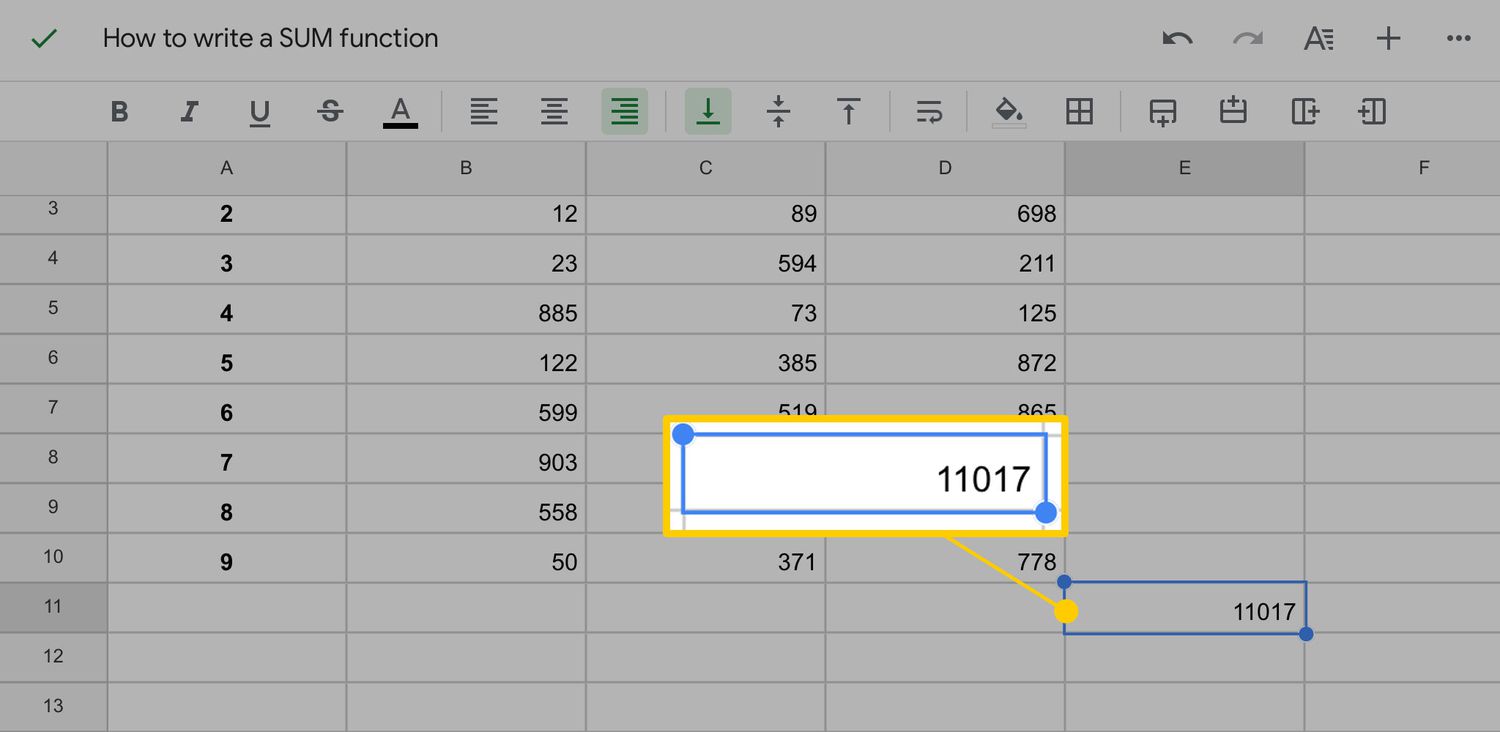
The SUM function in Google Sheets is a powerful tool that allows you to calculate the sum of a range of cells quickly and easily. It is especially useful when you need to add up a column or row of numbers or when you want to find the total value of a set of values.
To use the SUM function, you need to select the range of cells you want to add up. This can be done by clicking and dragging the cursor over the cells or by manually entering the range in the function. For example, if you have a column of numbers from A1 to A10 and you want to find their sum, you can use the SUM function like this: “=SUM(A1:A10)”. It will add up all the values in the range from A1 to A10 and display the total in the cell where you entered the function.
The SUM function can also be used to add up multiple ranges of cells. For example, you can use the function “=SUM(A1:A5, B1:B5)” to add up the values in both ranges A1 to A5 and B1 to B5. This is extremely handy when you have data distributed across different areas of your spreadsheet and want to find the cumulative sum.
Furthermore, the SUM function can be used with other functions and operators to perform more complex calculations. For instance, you can use it in combination with the AVERAGE function to find the sum of a range of cells divided by the count of cells in that range, giving you the average value.
Another useful feature of the SUM function is the ability to ignore non-numeric values within the range. If there are any cells with text or empty cells within the range, the SUM function will simply exclude them from the calculation, allowing you to get the sum of only the numeric values.
In addition to using the SUM function manually, you can also take advantage of the AutoSum feature in Google Sheets. Simply select the cell where you want to display the sum, click on the AutoSum icon (∑) in the toolbar, and it will automatically insert the SUM function with the range of the adjacent cells. This is a quick and convenient way to sum up your data without the need to type out the function manually.
Overall, the SUM function in Google Sheets is a valuable tool for summing up values and finding totals in your spreadsheets. Whether you need to add up a column of numbers or calculate cumulative sums from multiple ranges, the SUM function provides a straightforward and efficient solution.
Average Function
The AVERAGE function in Google Sheets is a powerful tool that allows you to calculate the average value of a range of cells quickly and accurately. It is particularly useful when you want to find the mean or average of a set of numbers.
To use the AVERAGE function, you simply need to select the range of cells you want to average. This can be done by clicking and dragging the cursor over the cells or by manually entering the range in the function. For example, if you have a column of numbers from A1 to A10 and you want to find their average, you can use the AVERAGE function like this: “=AVERAGE(A1:A10)”. The function will calculate the average of all the values in the range from A1 to A10 and display the result in the cell where you entered the function.
The AVERAGE function can also be used with multiple ranges of cells. For instance, if you have values in both ranges A1 to A5 and B1 to B5, you can use the function “=AVERAGE(A1:A5, B1:B5)” to calculate the average value across both ranges. This is particularly useful when your data is spread out across different areas of your spreadsheet, and you want to find the overall average.
In addition to calculating the average of a range of cells, the AVERAGE function can be combined with other functions and operators to perform more complex calculations. For example, you can use the function in combination with the SUM function to find the sum of a range of cells divided by the count of cells in that range. This will give you the average value of the range.
Another handy feature of the AVERAGE function is its ability to ignore non-numeric values within the range. If there are any cells with text or empty cells within the range, the AVERAGE function will simply exclude them from the calculation, ensuring that you get an accurate average of only the numeric values.
Like other functions in Google Sheets, the AVERAGE function can also be used with the AutoSum feature. By selecting the cell where you want to display the average, clicking on the AutoSum icon (∑) in the toolbar, and choosing “Average,” Google Sheets will automatically insert the AVERAGE function with the range of adjacent cells. This saves you time and effort, especially when you have a large dataset.
In summary, the AVERAGE function in Google Sheets is a powerful tool for calculating the average value of a range of cells. Whether you need to find the mean of a column of numbers or calculate the overall average from multiple ranges, the AVERAGE function provides a simple and reliable solution.
Count Function
The COUNT function in Google Sheets is a versatile tool that helps you count the number of cells in a range that contain numeric values. It is particularly useful when you want to keep track of entries or responses in a dataset or determine the number of cells that meet certain criteria.
To use the COUNT function, simply select the range of cells you want to count. This can be done by clicking and dragging the cursor over the cells or by manually entering the range in the function. For example, if you have a column of numbers from A1 to A10 and you want to count the number of values in that range, you can use the COUNT function like this: “=COUNT(A1:A10)”. The function will count the number of cells that contain numeric values in the range from A1 to A10 and display the result in the cell where you entered the function.
The COUNT function can also be used with multiple ranges of cells. If you have values in both ranges A1 to A5 and B1 to B5, for example, you can use the function “=COUNT(A1:A5, B1:B5)” to calculate the total count across both ranges. This is particularly useful when you have data distributed across different areas of your spreadsheet and want to find the cumulative count.
In addition to counting numeric values, the COUNT function can also be used to count cells that meet specific criteria. For example, if you want to count the number of cells in a range that are greater than a certain value, you can use the COUNT function in combination with the “>” operator. Similarly, you can use other comparison operators like “<", ">=”, “<=", or "<>” (not equal to) to count cells based on specific conditions.
Furthermore, the COUNT function automatically ignores empty cells and cells with text or non-numeric values within the range. This ensures that you get an accurate count of only the cells that meet your criteria. It is a convenient feature that saves you time and eliminates the need to manually filter out non-numeric values.
Lastly, just like other functions in Google Sheets, the COUNT function can also be used with the AutoSum feature. By selecting the cell where you want to display the count, clicking on the AutoSum icon (∑) in the toolbar, and selecting “Count,” Google Sheets will automatically insert the COUNT function with the range of adjacent cells. This makes counting cells even more effortless, especially when dealing with large datasets.
In summary, the COUNT function in Google Sheets is a valuable tool for counting cells that contain numeric values or meet specific criteria. Whether you need to keep track of entries or responses in a dataset or count cells based on conditions, the COUNT function provides a straightforward and efficient solution.
Min and Max Functions
The MIN and MAX functions in Google Sheets are powerful tools that help you find the minimum and maximum values in a range of cells, respectively. These functions are particularly useful when you need to identify the lowest and highest values in a dataset or make comparisons between values.
To use the MIN function, simply select the range of cells you want to find the minimum value of. This can be done by clicking and dragging the cursor over the cells or by manually entering the range in the function. For example, if you have a column of numbers from A1 to A10 and you want to find the minimum value in that range, you can use the MIN function like this: “=MIN(A1:A10)”. The function will identify the smallest value in the range from A1 to A10 and display the result in the cell where you entered the function.
Similarly, to use the MAX function, select the range of cells you want to find the maximum value of. Just like the MIN function, this can be done by clicking and dragging or by manually entering the range. For example, if you have a column of numbers from A1 to A10 and you want to find the maximum value in that range, you can use the MAX function like this: “=MAX(A1:A10)”. The function will identify the largest value in the range and display the result in the cell where you entered the function.
The MIN and MAX functions can also be used with multiple ranges of cells. If you have values in both ranges A1 to A5 and B1 to B5, for instance, you can use the functions “=MIN(A1:A5, B1:B5)” and “=MAX(A1:A5, B1:B5)” to calculate the overall minimum and maximum values across both ranges. This allows for easy comparison and analysis of values across different areas of your spreadsheet.
Another useful feature of the MIN and MAX functions is their ability to ignore non-numeric values within the range. If there are any cells with text or empty cells within the range, the functions will simply exclude them from the calculation, ensuring that you get accurate results based on numeric values only.
By using the MIN and MAX functions, you can quickly identify the smallest and largest values in a range of cells, making it easier to analyze data and make informed decisions. Whether you are working with sales figures, test scores, or any other numerical data, the MIN and MAX functions provide a convenient and efficient way to extract valuable insights from your dataset.
Advanced Functions
Google Sheets offers a range of advanced functions that can significantly enhance your data manipulation and analysis capabilities. These functions provide more complex calculations and allow you to perform tasks such as conditional statements, data lookup, combining text, and working with arrays. In this section, we will explore some of these advanced functions and their applications.
One of the most versatile advanced functions in Google Sheets is the IF function. This function allows you to evaluate a logical condition and return different values based on the result. For example, you can use the IF function to check if a student’s test score is above a certain threshold and assign a “Pass” or “Fail” label accordingly. The IF function is invaluable for creating dynamic formulas and performing calculations based on specific conditions.
The VLOOKUP function is another powerful tool that enables you to search for a value in a range and return a corresponding value from a different column. It is commonly used for data lookup and retrieval purposes. For instance, if you have a table with product names and prices, you can use the VLOOKUP function to search for a specific product name and return its corresponding price. The VLOOKUP function streamlines the process of finding specific information within large datasets.
The CONCATENATE function allows you to combine text strings from multiple cells into a single cell. This can be particularly useful when you want to create a personalized message or concatenate data from different sources. For example, you can use CONCATENATE to combine a customer’s first name, last name, and a greeting message to create a personalized email salutation.
Working with arrays can be simplified using the ARRAYFORMULA function. This function allows you to apply a formula or function to an entire range of cells instead of applying it to each cell individually. It reduces the need for repetitive copy-pasting of formulas. For instance, if you want to calculate the square of each number in a range, you can use ARRAYFORMULA to simplify the process and perform the calculation in a single step.
These advanced functions provide endless possibilities for data manipulation and analysis in Google Sheets. With the IF function, you can perform conditional calculations, while the VLOOKUP function enables efficient data lookup and retrieval. The CONCATENATE function makes it easy to combine text strings, and the ARRAYFORMULA function simplifies working with arrays. Mastery of these advanced functions can significantly improve your productivity and the quality of your spreadsheet work.
IF Function
The IF function in Google Sheets is a powerful tool that allows you to perform conditional calculations and make decisions based on specific criteria. It enables you to evaluate a logical condition and return different values depending on whether the condition is true or false. The IF function is particularly useful when you want to automate calculations, perform data validation, or apply conditional formatting based on specific conditions.
The basic syntax of the IF function consists of three parts: the logical condition, the value to return if the condition is true, and the value to return if the condition is false. For example, let’s say you have a dataset of test scores in column A, and you want to assign a “Pass” or “Fail” label based on a certain threshold value. You can use the IF function like this: “=IF(A1>=70, “Pass”, “Fail”)”. This function evaluates whether the test score in cell A1 is greater than or equal to 70. If it is true, it returns “Pass”; otherwise, it returns “Fail”.
The IF function can also be nested to evaluate more complex conditions. By combining multiple IF functions, you can create intricate logical statements. This allows you to handle multiple scenarios and perform calculations based on various conditions. For example, you can use nested IF functions to assign grades based on different score ranges, such as “A” for scores above 90, “B” for scores between 80 and 89, and so on.
In addition to using logical comparisons, you can also utilize logical operators like AND, OR, and NOT within the IF function to evaluate multiple conditions simultaneously. This enables you to create more sophisticated logical statements. For example, you can use the AND operator to check if a customer’s purchase amount exceeds a certain threshold and if their subscription is active before applying a discount.
Moreover, the IF function can be used in combination with other functions to perform more complex calculations. You can incorporate mathematical calculations, text concatenation, or other functions within the IF function to achieve customized outcomes. This flexibility allows you to create dynamic formulas and automate calculations based on specific conditions.
The IF function is an invaluable tool for making decisions and performing calculations based on specific conditions. Whether you need to assign labels, calculate incentives, validate data, or apply conditional formatting, the IF function provides a flexible and efficient solution. Mastering the IF function allows you to automate processes and streamline your spreadsheet work, making your data analysis tasks more efficient and accurate.
VLOOKUP Function
The VLOOKUP function in Google Sheets is a powerful tool that allows you to search for a specific value in a range of cells and retrieve a corresponding value from a different column. It is commonly used for data lookup, retrieval, and analysis purposes. The VLOOKUP function is particularly useful when you have large datasets and need to find specific information quickly and accurately.
The basic syntax of the VLOOKUP function consists of four parts: the search key, the range to search in, the column index from which to retrieve the value, and an optional Boolean value for exact or approximate match. For example, let’s say you have a table with product names in column A and corresponding prices in column B, and you want to find the price of a specific product. You can use the VLOOKUP function like this: “=VLOOKUP(“Product Name”, A:B, 2, false)”. This function searches for the value “Product Name” in column A, retrieves the corresponding value from column B (which is the second column in the range), and returns the price.
In addition to exact match searches, the VLOOKUP function also allows for approximate match searches by setting the last argument to “true” or “1”. This is useful when you work with sorted data and want to find the closest value that is less than or equal to the search key. However, it is important to note that for approximate matches, the search column must be sorted in ascending order.
The VLOOKUP function can also be used with multiple criteria by combining it with other functions like CONCATENATE or TEXTJOIN. By concatenating or joining multiple values, you can create a compound search key and retrieve more specific information. This is particularly useful when you have composite keys or when you need to perform lookups based on multiple conditions.
Furthermore, the VLOOKUP function also has an option to display an error value if the search key is not found in the range. This prevents incorrect or misleading results when performing lookups and provides an indication that the search key doesn’t exist in the dataset.
By utilizing the VLOOKUP function, you can easily retrieve information from large datasets, perform data analysis, and make quick comparisons. Whether you need to find prices, match customer names, or retrieve any other data based on specific criteria, the VLOOKUP function in Google Sheets provides a convenient and efficient solution.
CONCATENATE Function
The CONCATENATE function in Google Sheets is a handy tool that allows you to combine text strings from multiple cells into a single cell. It is particularly useful when you want to create a unified message, concatenate data from different sources, or format data in a specific way.
The basic syntax of the CONCATENATE function involves listing the text strings or cell references you want to combine within the function’s parentheses. For example, if you have the first name in cell A1 and the last name in cell B1, you can use the CONCATENATE function like this: “=CONCATENATE(A1, ” “, B1)”. This function will combine the contents of cell A1 and a space character with the contents of cell B1, resulting in the full name displayed in the cell where you entered the function.
In addition to directly inputting text strings, you can also incorporate cell references, numbers, or other functions within the CONCATENATE function. This allows for dynamic concatenation based on changing values or calculations. For example, you can concatenate a customer’s name, order number, and order date to create a personalized order confirmation message by using cell references and the TEXT function to format the date.
The CONCATENATE function also enables you to add static text, such as spaces, punctuation, or formatting characters, within the resulting text string. By including these static elements within quotation marks, you can control the format and appearance of the concatenated text. For example, you can add a comma and a space between first and last names by using the CONCATENATE function like this: “=CONCATENATE(A1, “, “, B1)”.
In addition to the CONCATENATE function, Google Sheets also provides an alternative operator for concatenation: the ampersand (&). This operator can achieve the same result as the CONCATENATE function and is often used for concatenation in a more concise and intuitive manner. The example mentioned earlier can also be written as “=A1 & “, ” & B1″.
By leveraging the CONCATENATE function in Google Sheets, you can easily merge text strings, combine data from different cells, and create dynamic messages or labels. Whether you need to concatenate names, addresses, or other sets of data, the CONCATENATE function provides a flexible and efficient solution.
ARRAYFORMULA Function
The ARRAYFORMULA function in Google Sheets is a powerful tool that allows you to apply a formula or function to an entire range of cells at once. It eliminates the need to manually copy and paste formulas, saving you time and effort when working with large datasets or performing complex calculations.
When using the ARRAYFORMULA function, you can input the formula or function you want to apply to the first cell of the range. Google Sheets will automatically extend the formula or function to all the cells in the specified range, providing seamless calculations or operations across multiple cells.
One of the primary benefits of the ARRAYFORMULA function is its ability to perform calculations on arrays of data. By using this function, you can work with multiple values or ranges simultaneously, performing operations such as addition, multiplication, or even more complex calculations. This is particularly useful when dealing with large datasets or when you want to perform calculations that involve multiple variables.
The ARRAYFORMULA function also allows you to combine other functions within it. This enables you to create more advanced and sophisticated calculations by nesting or combining functions together. You can apply multiple functions to an entire range of cells with a single formula, resulting in improved efficiency and readability.
In addition, the ARRAYFORMULA function is often used in conjunction with other Google Sheets functions, such as SUM, AVERAGE, or COUNT, to process data across multiple cells or ranges. It simplifies the process of working with arrays and provides a more streamlined approach to data manipulation and analysis.
It’s important to note that the ARRAYFORMULA function operates differently from regular formulas. For instance, it will automatically adjust the range references when new data is added to the sheet. This dynamic behavior ensures that your formulas remain accurate and up-to-date as you work with your spreadsheet.
The ARRAYFORMULA function in Google Sheets is a powerful tool that allows you to apply a formula or function to an entire range of cells. It simplifies complex calculations, speeds up data manipulation tasks, and ensures the accuracy and consistency of your formulas. Whether you need to perform calculations on large datasets, work with arrays of data, or streamline your spreadsheet work, the ARRAYFORMULA function provides a versatile and efficient solution.
Tips and Tricks
When working with Google Sheets, there are many helpful tips and tricks that can enhance your productivity and make your spreadsheet work more efficient and effective. Here are some valuable tips and tricks to consider:
- Using Absolute and Relative References: When creating formulas, you can use absolute references (e.g., $A$1) to lock the reference to a specific cell, or relative references (e.g., A1) to allow the reference to adjust when copied to other cells. Understanding how to use these references can save you time and prevent errors in your calculations.
- Using Named Ranges: Assigning names to specific ranges of cells can make your formulas more readable and easier to manage. Instead of referencing cells using their coordinates, you can use descriptive names to improve the clarity and understanding of your formulas.
- Using Data Validation: Data validation is a powerful feature that allows you to define specific rules or criteria for the data entered into a cell. By setting data validation rules, you can ensure data accuracy and prevent errors in your spreadsheets. It’s particularly useful when creating input forms or when sharing spreadsheets with others.
- Utilizing Filters and Sorting: Google Sheets offers an array of filtering and sorting options that allow you to manipulate and analyze your data. By using filters, you can quickly extract specific subsets of data based on different criteria. Sorting your data enables you to arrange it in ascending or descending order, making it easier to identify patterns and trends.
- Conditional Formatting: Conditional formatting is a powerful tool that lets you apply formatting rules to cells based on specific conditions. It allows you to highlight data, add color scales or icons, and visually represent patterns in your dataset. Conditional formatting can enhance data visualization and make it easier to interpret your data.
- Collaboration and Sharing: Google Sheets provides excellent collaboration features, allowing multiple users to work on the same spreadsheet simultaneously. Take advantage of the real-time editing and commenting features to collaborate effectively with colleagues or teammates. Additionally, you can control access and permission levels when sharing your spreadsheets to ensure data security.
By utilizing these tips and tricks, you can make the most out of Google Sheets and improve your overall spreadsheet workflow. From optimizing formulas to enhancing data visualization and collaboration, these techniques will help you achieve greater efficiency and effectiveness in your data manipulation and analysis tasks.
Using Absolute and Relative References
When working with formulas in Google Sheets, understanding the concept of absolute and relative references is crucial. Absolute and relative references define how cell references in a formula behave when the formula is copied and applied to other cells. Mastering these reference types can significantly improve your efficiency and accuracy when working with spreadsheets.
Relative References: By default, cell references in a formula are relative. This means that when you copy a formula to another cell, the references will adjust based on their relative position to the new cell. For example, if you copy a formula that references cell A1 to cell B2, the formula will adjust to reference cell B2 instead of A1. Relative references are denoted by their column letter and row number without any dollar signs.
Absolute References: In some cases, you may want to lock a reference to a specific cell, regardless of where the formula is copied. Absolute references allow you to achieve this. To create an absolute reference, you need to add dollar signs before the column letter, row number, or both. For example, $A$1 is an absolute reference that always refers to cell A1, regardless of where the formula is copied.
Mixed References: In certain scenarios, you may need both relative and absolute references. To create a mixed reference, you can lock either the row or column while keeping the other part of the reference relative. For example, $A1 is a mixed reference that allows the column to change when the formula is copied horizontally but keeps the row fixed at row 1.
Using absolute references is particularly useful when referencing fixed values or when you want to apply the same formula to a specified range. On the other hand, relative references are handy when you want to perform calculations based on the relative position of data across multiple cells or ranges.
Another useful technique is utilizing the F4 key to quickly switch between absolute and relative references. When editing a formula, pressing F4 will cycle through different reference types for the selected cell or range. This shortcut can save valuable time when you have complex formulas with various reference types.
Understanding how to use absolute and relative references effectively can prevent errors and streamline your spreadsheet work. Whether you are working with large datasets, performing calculations across multiple cells, or creating dynamic formulas, mastering these reference types will significantly enhance your efficiency and accuracy in Google Sheets.
Using Named Ranges
In Google Sheets, using named ranges is a powerful technique that can enhance the readability, manageability, and functionality of your formulas. Instead of referring to cells by their coordinate references, you can assign descriptive names to specific ranges of cells. This makes your formulas more intuitive, easier to understand, and less prone to errors.
Creating Named Ranges: To create a named range, you can go to the “Data” menu, select “Named ranges,” and then choose “Define a named range.” Alternatively, you can use the shortcut Ctrl + Shift + F3. Enter the desired name for the range and specify the range of cells you want to include. You can also create dynamic named ranges using formulas to automatically adjust the range based on changing data.
Using Named Ranges in Formulas: Once you have created a named range, you can use it in your formulas instead of using cell references. For example, instead of writing “=SUM(A1:A10)”, you can write “=SUM(Sales)”. This not only makes the formula more readable but also makes it easier to understand the purpose of the formula at a glance. If you need to update the range, you can simply modify the named range definition instead of updating each formula individually.
Benefits of Named Ranges: Using named ranges brings several benefits. It improves the clarity of your formulas by clearly indicating the purpose and meaning of the referenced data. Named ranges also make your formulas more resilient to changes in spreadsheet structure when inserting or deleting columns or rows. Furthermore, it simplifies formula auditing and troubleshooting by providing more meaningful cell references in error messages.
Managing Named Ranges: Google Sheets provides features to manage your named ranges. You can access the named ranges manager by going to the “Data” menu and selecting “Named ranges.” From there, you can edit the range, rename it, or delete it if it’s no longer needed. Additionally, you can use the named ranges manager to view and navigate through all named ranges within your spreadsheet.
Named ranges are especially useful when working with complex formulas, large datasets, or when collaborating with others. They provide a clear and meaningful way to refer to ranges of cells, improving the readability and understanding of your formulas. By utilizing named ranges effectively, you can create more maintainable and error-resistant spreadsheets in Google Sheets.
Using Data Validation
Data validation is a powerful feature in Google Sheets that allows you to define specific rules or criteria for the data entered into a cell. It helps ensure data accuracy, consistency, and integrity by validating input based on predefined conditions. By utilizing data validation effectively, you can minimize errors, improve data quality, and make your spreadsheets more reliable.
Creating Data Validation: To apply data validation to a cell or range, select the cell(s), go to the “Data” menu, and choose “Data validation.” This will open a dialog box where you can define the validation criteria. You can choose from various validation options such as numbers, text, dates, and custom formulas. You can set conditions such as greater than or equal to, list of items, range of dates, or specific custom rules based on your needs.
Benefits of Data Validation: Data validation provides several benefits. It ensures that the data entered meets specific criteria, such as within a certain range or format, reducing the chance of inaccurate or invalid data being entered. This is particularly useful for preventing data entry errors by users or when you want to enforce specific rules or standards for data collection.
Error Alert and Custom Messages: Data validation also allows you to display an error alert or custom message when the entered data violates the validation rules. The error alert can be customized to provide instructions or explanations about the required data format. This helps users understand and rectify any data entry mistakes, leading to better data quality and consistency.
List of Items: One useful data validation option is the ability to create a dropdown list of items. This allows users to select values from a predefined list, ensuring that the entered data is limited to specific options. Dropdown lists help standardize data entry, make it easier for users to select the correct value, and minimize typing errors.
Conditional Data Validation: Google Sheets also provides the ability to create data validation that is based on other cell values or formulas. This enables you to create dynamic data validation, where the allowed values change according to certain conditions. It is particularly useful when you want to create complex data entry rules or when the valid choices depend on other factors in the spreadsheet.
Managing Data Validation: You can manage and modify existing data validation rules by selecting the cell(s) with data validation, going to the “Data” menu, and choosing “Data validation.” From there, you can adjust the criteria, modify the error alert, or remove the data validation altogether.
By employing data validation in Google Sheets, you can enforce data integrity, enhance data accuracy, and streamline data entry processes. Whether you need to restrict data to specific formats, provide dropdown options, or validate entries based on custom rules, data validation is a powerful tool that ensures the reliability and consistency of your data.
Conclusion
In conclusion, Google Sheets offers a wide range of features and functions that can greatly enhance your productivity and efficiency when working with spreadsheets. From the basic functions like SUM, AVERAGE, COUNT, MIN, and MAX to the more advanced functions like IF, VLOOKUP, CONCATENATE, and ARRAYFORMULA, these tools provide the necessary means to perform calculations, analyze data, and create dynamic formulas.
By utilizing absolute and relative references, you can control how cell references behave when formulas are copied and applied to different cells. This ensures accuracy and consistency when working with large data sets and performing complex calculations.
Named ranges provide a more intuitive and readable way to refer to ranges of cells in your formulas, making your spreadsheets easier to understand and maintain. Data validation is a powerful tool to enforce data accuracy and consistency by defining specific rules for data entry and display informative error alerts when the entered data is invalid.
Moreover, Google Sheets offers collaborative features that allow multiple users to work on the same spreadsheet simultaneously, enabling seamless teamwork and effective collaboration.
Implementing these techniques and adopting best practices can significantly improve your productivity, accuracy, and efficiency when working with Google Sheets. By leveraging the power of these features, you can manipulate and analyze data effectively, automate calculations, and create more meaningful and insightful spreadsheets.
Whether you are a professional managing complex data analysis or a student organizing coursework, Google Sheets provides a powerful platform that caters to a wide range of spreadsheet needs. So dive in, explore the functionalities, and make the most of Google Sheets to boost your productivity and achieve your spreadsheet goals.