How To Insert Dates In Google Sheets

Introduction

Welcome to this tutorial on how to insert dates in Google Sheets! Dates are an integral part of any spreadsheet, and Google Sheets provides several methods to input and manipulate dates. Whether you need to track project milestones, plan events, or simply keep track of important dates, knowing how to insert and work with dates in Google Sheets is a valuable skill.

Accurately recording dates in your spreadsheet ensures that you have a clear timeline of events, and it also allows you to perform various calculations and analysis based on dates. Whether you are a beginner or an experienced user, this guide will walk you through different methods to insert dates, so you can choose the one that suits your needs best.

From manually typing the date to using functions like TODAY(), DATE(), or EOMONTH(), we will explore a variety of techniques to input dates accurately and efficiently. Additionally, we will cover how to format dates and apply various date-related calculations to enhance your data analysis.

No matter the nature of your spreadsheet or the purpose of your date entries, this tutorial will equip you with the necessary knowledge to handle dates effectively in Google Sheets. So, let’s get started with the different methods of inserting dates and unlock the potential of your spreadsheet!

Method 1: Manually Typing the Date

The most straightforward way to insert a date in Google Sheets is by manually typing it. To manually enter a date, select the cell where you want to input the date, and then simply type the date in the desired format. Google Sheets recognizes common date formats such as “mm/dd/yyyy,” “dd/mm/yyyy,” and “yyyy/mm/dd.”

When manually typing a date, make sure it is entered correctly to avoid any data entry errors. Take note of the desired date format and include the necessary separators (slashes, hyphens, or periods) between the day, month, and year. For example, if you want to enter June 1, 2022, you can type “06/01/2022” or “1-Jun-2022” depending on your preferred format.

It’s important to note that Google Sheets automatically recognizes and converts valid date entries, so you don’t have to worry about the formatting unless you want to apply a specific style to the cell containing the date.

To manually enter a date in Google Sheets:

1. Select the desired cell where you want to insert the date.
2. Type the date using the desired format (e.g., “mm/dd/yyyy” or “dd-mm-yyyy”).
3. Press Enter or move to another cell to confirm the date entry.

Manually typing the date is a quick and easy method to insert dates, especially when you only have a few dates to input. However, it may not be the most efficient method if you need to work with a large volume of dates or if you require dates to be automatically updated.

Now that you know how to manually enter dates in Google Sheets, let’s explore other methods that can help automate date entries and calculations.

Method 2: Using the TODAY() Function

One handy function in Google Sheets for inserting the current date is the TODAY() function. The TODAY() function automatically inserts today’s date into a cell, which can be useful for tracking the current date or for timestamping when a particular event occurred.

To use the TODAY() function:

1. Select the cell where you want to insert the current date.
2. Type =TODAY() or simply click on the “Functions” button (Σ) in the formula bar and select “Date” > “Today”.
3. Press Enter or move to another cell to apply the function and display the current date.

Whenever the spreadsheet recalculates, the cell containing the TODAY() function will display the updated current date. This makes it convenient for automatically tracking the progress of time without the need for manual intervention.

It’s important to note that when using the TODAY() function, the date is always displayed in the default date format set in your Google Sheets settings. If you want to change the format, you can apply the desired date format to the cell with the TODAY() function using the format options in the toolbar.

The TODAY() function is a powerful tool for inserting and tracking the current date in Google Sheets. However, it updates every time the spreadsheet recalculates, which may not be ideal for historical record-keeping or situations where you need to freeze the date to a particular value.

Now that you know how to use the TODAY() function to insert the current date, let’s explore other methods to input and manipulate dates in Google Sheets.

Method 3: Using the DATEVALUE() Function

If you have dates stored as text or in a different format that Google Sheets does not recognize, you can use the DATEVALUE() function to convert them into proper date values. This function allows you to transform text representations of dates into the equivalent numerical value that Google Sheets recognizes as a date.

To use the DATEVALUE() function:

1. Select the cell where you want to insert the converted date.
2. Type =DATEVALUE(“date”) or simply click on the “Functions” button (Σ) in the formula bar and select “Date” > “DateValue”. Replace “date” with the cell reference or the text representation of the date you want to convert. For example, =DATEVALUE(“2/15/2022”) or =DATEVALUE(A2) if the date is in cell A2.
3. Press Enter or move to another cell to apply the function and display the converted date.

The DATEVALUE() function converts the text representation of a date into a numerical value that Google Sheets recognizes as a date, allowing you to perform date-related calculations or apply date formatting.

It’s important to note that the text representation of the date should be in a format that Google Sheets recognizes. If the dates are in a different format, you may need to adjust the format to match Google Sheets’ default date format or employ additional formulas to extract and rearrange the date elements before using the DATEVALUE() function.

The DATEVALUE() function is a useful tool for converting text representations of dates into proper date values in Google Sheets. By utilizing this function, you can ensure accurate calculations and formatting for your date data.

Now that you know how to use the DATEVALUE() function, let’s explore other methods to input and manipulate dates in Google Sheets.

Method 4: Using the DATE() Function

The DATE() function in Google Sheets allows you to create a date by specifying the year, month, and day as separate arguments. This is especially useful when you have separate columns or cells containing the year, month, and day values, and you want to combine them into a single date.

To use the DATE() function:

1. Select the cell where you want to insert the combined date.
2. Type =DATE(year, month, day) or simply click on the “Functions” button (Σ) in the formula bar and select “Date” > “Date”. Replace year, month, and day with the respective cell references or numerical values. For example, =DATE(A2, B2, C2) if the year is in cell A2, the month is in cell B2, and the day is in cell C2.
3. Press Enter or move to another cell to apply the function and display the combined date.

The DATE() function combines the year, month, and day arguments to create a valid date value in Google Sheets. This function is particularly useful for situations where the date components are stored separately, such as in different columns or cells.

It’s important to note that the DATE() function requires valid numerical values for the year, month, and day. You can use cell references or directly enter numerical values for these arguments. Make sure the arguments are correctly formatted to avoid errors.

The DATE() function enables you to quickly create dates by combining separate year, month, and day values. This can be beneficial when working with date data split across different columns or cells.

Now that you know how to use the DATE() function, let’s explore other methods to input and manipulate dates in Google Sheets.

Method 5: Using the NOW() Function

The NOW() function in Google Sheets allows you to insert the current date and time into a cell. Similar to the TODAY() function, the NOW() function updates automatically whenever the spreadsheet recalculates, providing an up-to-date timestamp.

To use the NOW() function:

1. Select the cell where you want to insert the current date and time.
2. Type =NOW() or simply click on the “Functions” button (Σ) in the formula bar and select “Date” > “Now”.
3. Press Enter or move to another cell to apply the function and display the current date and time.

The cell containing the NOW() function will display the current date and time, including the timestamp of when it was last recalculated. This can be useful for tracking events or keeping a record of when specific actions occurred.

It’s important to note that when using the NOW() function, the date and time are displayed in the default date and time format set in your Google Sheets settings. If you want to change the format, you can apply the desired date and time formatting to the cell with the NOW() function using the format options in the toolbar.

The NOW() function is a versatile tool for inserting the current date and time, providing a real-time timestamp. Though it recalculates whenever the spreadsheet is recalculated, it can be valuable in scenarios where you need to track the current date and time dynamically.

Now that you know how to use the NOW() function to insert the current date and time, let’s explore another method to input and manipulate dates in Google Sheets.

Method 6: Using the NOW() Function with Formatting

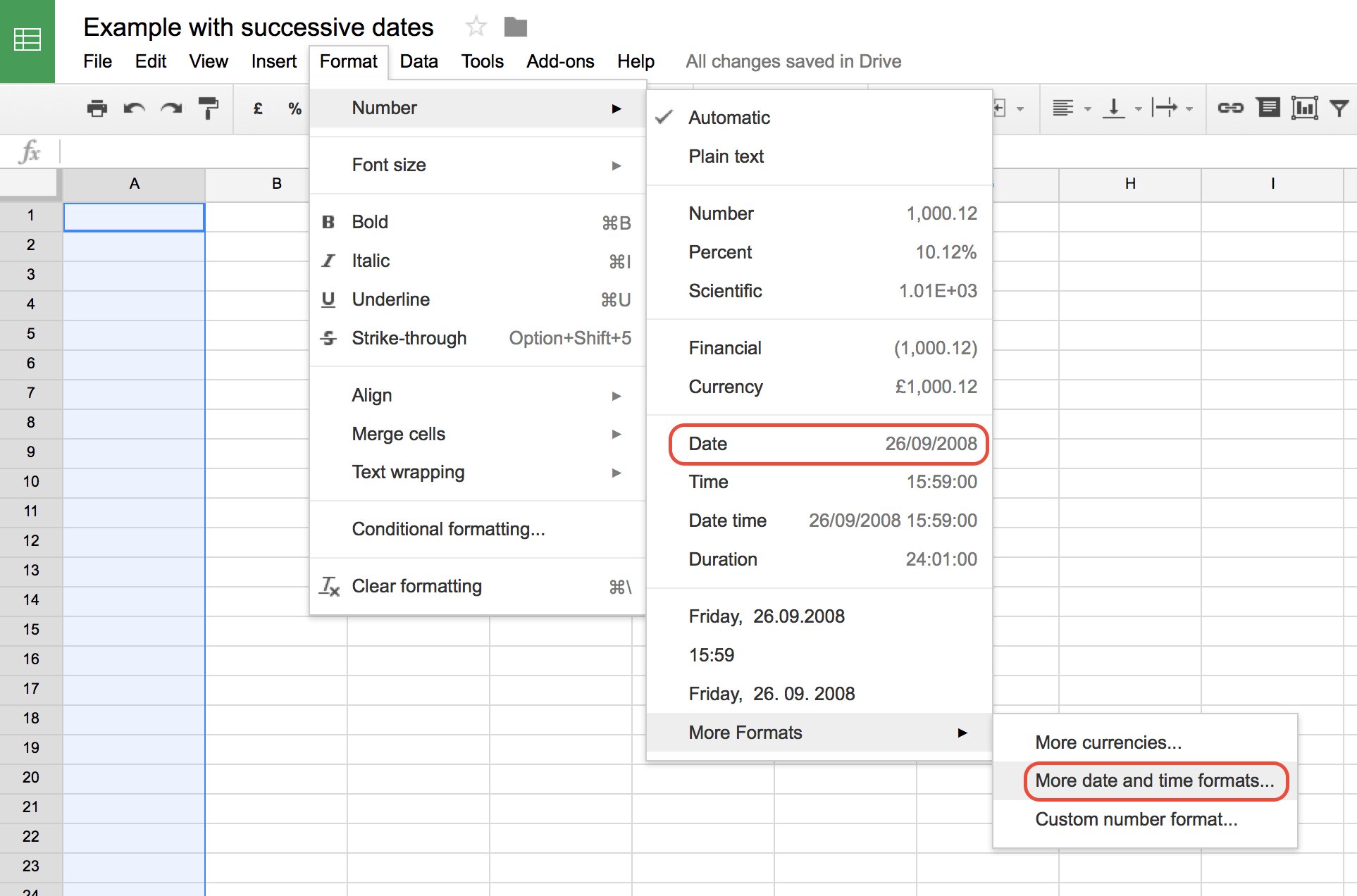
When using the NOW() function to insert the current date and time in Google Sheets, you can apply formatting options to customize the display of the date and time. This allows you to present the timestamp in a format that suits your preferences or aligns with the requirements of your spreadsheet.

To use the NOW() function with formatting:

1. Select the cell where you want to insert the formatted current date and time.
2. Type =NOW() or simply click on the “Functions” button (Σ) in the formula bar and select “Date” > “Now”.
3. Apply the desired formatting to the cell using the formatting options in the toolbar. You can choose from a variety of date and time formats or even create a custom format.
4. Press Enter or move to another cell to apply the function and display the current date and time in the formatted style.

By applying formatting options, you can modify the display of the current date and time to include or exclude specific information such as day, month, year, hour, minute, or second. You can also adjust the order of these elements and add separators or text symbols to enhance readability.

Formatting options in Google Sheets allow you to customize the appearance of the date and time to suit your specific needs. Simply select the desired format from the formatting options menu, and the cell will display the current date and time accordingly.

Keep in mind that the NOW() function with formatting will continue to update whenever the spreadsheet recalculates, displaying the most recent date and time according to the applied formatting.

Now that you know how to use the NOW() function with formatting to insert the current date and time, let’s explore another method to input and manipulate dates in Google Sheets.

Method 7: Using the WEEKDAY() Function

The WEEKDAY() function in Google Sheets allows you to determine the day of the week for a given date. This function returns a numerical value representing the day of the week, with Sunday being 1 and Saturday being 7. It can be useful for analyzing data based on the day of the week or performing date-related calculations.

To use the WEEKDAY() function:

1. Select the cell where you want to display the day of the week.
2. Type =WEEKDAY(date) or simply click on the “Functions” button (Σ) in the formula bar and select “Date” > “Weekday”. Replace “date” with the cell reference or the date value for which you want to determine the day of the week. For example, =WEEKDAY(A2) if the date is in cell A2.
3. Press Enter or move to another cell to apply the function and display the day of the week as a numerical value.

The WEEKDAY() function returns a numerical value indicating the day of the week for the specified date. You can use this value in formulas or further format it to display the actual day name if desired.

It’s important to note that the WEEKDAY() function assigns Sunday as the first day of the week and Saturday as the last day. If you prefer a different configuration, you can adjust it by using additional functions and formulas in conjunction with the WEEKDAY() function.

The WEEKDAY() function provides a simple yet effective way to determine the day of the week for a given date. By leveraging this function, you can gain insights into trends or patterns based on the specific day of the week.

Now that you know how to use the WEEKDAY() function, let’s explore another method to input and manipulate dates in Google Sheets.

Method 8: Using the EDATE() Function

The EDATE() function in Google Sheets allows you to add or subtract a specified number of months from a given date. This function is particularly useful when you need to calculate future or past dates based on the original date.

To use the EDATE() function:

1. Select the cell where you want to display the calculated date.
2. Type =EDATE(start_date, months) or simply click on the “Functions” button (Σ) in the formula bar and select “Date” > “EDate”. Replace “start_date” with the cell reference or the initial date, and “months” with the number of months to add or subtract. For example, =EDATE(A2, 6) if the start date is in cell A2, and you want to add 6 months.
3. Press Enter or move to another cell to apply the function and display the calculated date.

The EDATE() function adds or subtracts the specified number of months from the start date to calculate the resulting date. This allows you to easily determine future or past dates without manually adjusting each date individually.

It’s important to note that the EDATE() function works with whole months, so if you add or subtract a partial month, it will adjust the date accordingly. For example, adding 1 month to January 31 will result in February 28 (or February 29 in a leap year).

The EDATE() function is a powerful tool for calculating dates based on an initial date and a specified number of months. By using this function, you can automate the process of determining future or past dates in your spreadsheet.

Now that you know how to use the EDATE() function, let’s explore another method to input and manipulate dates in Google Sheets.

Method 9: Using the EOMONTH() Function

The EOMONTH() function in Google Sheets allows you to determine the last day of the month for a specified date. This function is particularly useful when you need to calculate deadlines or track monthly progress based on the end date of each month.

To use the EOMONTH() function:

1. Select the cell where you want to display the last day of the month.
2. Type =EOMONTH(start_date, months) or simply click on the “Functions” button (Σ) in the formula bar and select “Date” > “Eomonth”. Replace “start_date” with the cell reference or the initial date, and “months” with the number of months forward or backward from the start date. For example, =EOMONTH(A2, 2) if the start date is in cell A2, and you want to calculate the last day of the month 2 months later.
3. Press Enter or move to another cell to apply the function and display the last day of the month.

The EOMONTH() function returns the last day of the month for the specified date and the specified number of months. This function is particularly useful for calculating due dates or determining the end of a specific billing or reporting period.

It’s important to note that the EOMONTH() function works with whole months, so if you add or subtract a partial month, it will adjust the date accordingly. For example, adding 1 month to January 31 will result in February 28 (or February 29 in a leap year).

The EOMONTH() function simplifies the task of determining the last day of the month for a given date. By utilizing this function, you can automate the process of calculating end-of-month dates in your spreadsheet.

Now that you know how to use the EOMONTH() function, let’s explore another method to input and manipulate dates in Google Sheets.

Method 10: Using the WORKDAY() Function

The WORKDAY() function in Google Sheets allows you to calculate a future or past working date by excluding weekends and specified holidays. This function is particularly useful when you need to determine project deadlines or estimate delivery dates based on working days.

To use the WORKDAY() function:

1. Select the cell where you want to display the calculated working date.
2. Type =WORKDAY(start_date, days, [holidays]) or simply click on the “Functions” button (Σ) in the formula bar and select “Date” > “Workday”. Replace “start_date” with the cell reference or the initial date, “days” with the number of working days to add or subtract, and [holidays] with an optional range of cells containing holiday dates (if applicable). For example, =WORKDAY(A2, 10, B2:B5) if the start date is in cell A2, you want to add 10 working days, and the holiday dates are in the range B2:B5.
3. Press Enter or move to another cell to apply the function and display the calculated working date.

The WORKDAY() function calculates the working date by excluding weekends and any specified holiday dates. It allows you to determine future or past working dates accurately, considering your organization’s or country’s specific holidays.

It’s important to note that weekends are automatically excluded when using the WORKDAY() function, based on your Google Sheets settings, where Saturday and Sunday are considered non-working days. Additionally, you can provide a range of cells containing holiday dates to exclude those dates from the calculation.

The WORKDAY() function is a powerful tool for calculating working dates based on a starting date and the number of working days to add or subtract. By leveraging this function, you can accurately estimate project timelines or delivery dates that align with working days.

Now that you know how to use the WORKDAY() function, let’s explore other methods to input and manipulate dates in Google Sheets.

Conclusion

Google Sheets provides a range of methods to insert and manipulate dates, allowing you to effectively work with date-related data in your spreadsheets. From manually typing the date to utilizing functions like TODAY(), DATEVALUE(), EDATE(), and WORKDAY(), each method offers unique ways to handle dates based on your specific needs.

When manually entering dates, ensure that you use the correct format and separators to accurately represent the date. Additionally, the TODAY() function is a useful tool for automatically inserting the current date, while the DATEVALUE() function allows you to convert text representations of dates into valid date values.

By using functions like DATE(), NOW(), and EOMONTH(), you can manipulate dates to create customized calculations and track various time-based events. The WEEKDAY() function helps determine the day of the week for a given date, while the WORKDAY() function calculates working dates considering weekends and specified holidays.

Remember to format the dates according to your preference using the formatting options available in Google Sheets. This allows you to present the dates in a visually appealing format that suits your needs and improves data visibility.

Whether you need to track project milestones, plan events, or analyze data based on dates, mastering the various methods to manipulate dates in Google Sheets is essential. By utilizing these techniques, you can streamline your data management and enhance your productivity.

Now that you have a solid understanding of the different methods available, you can confidently work with dates in Google Sheets and efficiently handle date-related tasks in your spreadsheets.