How Do You Freeze A Row In Google Sheets

Introduction

Welcome to the world of Google Sheets, where you can effortlessly organize and analyze your data. Whether you are a student, a professional, or a business owner, you have probably encountered the need to freeze rows in Google Sheets at some point. Freezing a row allows you to keep important information visible while scrolling through large datasets.

Imagine you have a spreadsheet filled with sales data for the past year, and you want to keep the header row in view while scrolling through the rest of the data. This is where freezing a row becomes incredibly useful. By freezing a row, you can keep it fixed at the top of the sheet, making your work much more efficient.

In this article, we will walk you through the process of freezing a row in Google Sheets. Whether you are a beginner or an experienced Sheets user, we’ve got you covered. So, let’s dive in and learn how to freeze rows in Google Sheets!

Why Freeze Rows in Google Sheets

Before we delve into the specifics of how to freeze rows in Google Sheets, let’s take a moment to understand the importance of this feature. Freezing rows in Google Sheets can greatly enhance your productivity and make working with large datasets a breeze. Here are a few reasons why you might want to consider freezing rows:

1. Improved Data Analysis: When dealing with large datasets, it can be challenging to keep track of the column headers or other important information as you scroll. By freezing rows, you can ensure that the headers are always visible, making it easier to understand and analyze your data.
2. Easier Navigation: If you have a spreadsheet with multiple sheets or tabs, freezing rows can help you navigate between different sections more smoothly. The frozen row will remain visible even as you switch between tabs, providing a constant point of reference.
3. Efficient Collaboration: When collaborating with others on a Google Sheet, freezing rows can enhance communication and reduce errors. By keeping important information fixed at the top, you can minimize the chances of accidental edits or misinterpretation of data.
4. Presentation-Ready Sheets: If you plan to share or present your Google Sheet, freezing rows can give it a more polished and professional look. By preventing the headers from scrolling out of view, you can create a clean and presentable spreadsheet that is easy to read and understand.

Now that we’ve explored the benefits of freezing rows in Google Sheets, let’s move on to the practical steps of how to actually freeze a row. By following a few simple instructions, you’ll be able to master this feature and take your data management skills to the next level.

Freezing a Row in Google Sheets

Now let’s get down to the nitty-gritty of freezing a row in Google Sheets. The process is remarkably straightforward, and you’ll be able to do it in just a few simple steps:

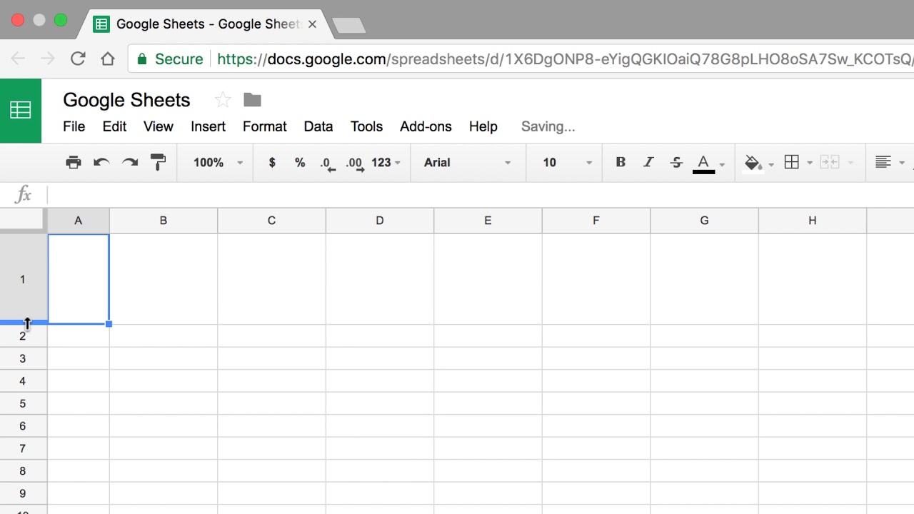
1. Step 1: Open Google Sheets: Log in to your Google account and navigate to Google Sheets. If you don’t have a sheet open, create a new one by clicking on the “+ New” button in your Google Drive.
2. Step 2: Select the Row to Freeze: Move your cursor to the row you want to freeze. You can either click on the row number on the left-hand side or simply click and drag to select multiple rows.
3. Step 3: Freeze the Row: With the desired row(s) selected, navigate to the “View” menu at the top of the screen. From the drop-down menu, choose “Freeze” followed by “1 row” (or the number of rows you selected).
4. Step 4: Adjust the Frozen Row: Once you have frozen the row, you may want to customize and adjust its appearance. To do this, click and drag the line below the frozen row to resize it or right-click on the row number and choose “Row height” to set a specific height.

That’s it! You’ve successfully frozen a row in Google Sheets. Now, as you scroll through your sheet, the frozen row will remain fixed at the top, allowing you to easily reference the information contained within it.

It’s worth noting that freezing rows in Google Sheets is not limited to just the top row. You can freeze multiple rows by selecting them before applying the freeze command. This can be especially useful if you have multiple header rows or if you want to keep certain information constantly in view.

Now that you know how to freeze rows in Google Sheets, let’s explore a few additional tips and tricks that can further enhance your experience with this powerful spreadsheet tool.

Step 1: Open Google Sheets

To begin the process of freezing a row in Google Sheets, you’ll first need to open the Google Sheets application. Here’s how you can do it:

1. Launch Google Sheets: Open your preferred web browser and go to the Google Sheets website. Alternatively, you can access Google Sheets through the Google Drive application.
2. Sign in to your Google account: If you’re not already signed in, enter your Google account credentials to log in. If you don’t have a Google account, you can create one for free.
3. Create a new sheet or open an existing one: Once you’re signed in, you have the option to create a new sheet by clicking on the “+ New” button and selecting “Google Sheets” or open an existing sheet from your Google Drive by clicking on it.

Google Sheets is a powerful and intuitive tool that allows you to manage and analyze your data with ease. It provides a range of features that can simplify your workflow, and freezing rows is just one of them.

Keep in mind that Google Sheets is a cloud-based application, which means that all your work is automatically saved as you go. This ensures that you never lose your progress, and you can access your sheets from any device with an internet connection.

Now that you’ve opened Google Sheets, you’re ready to move on to the next step and select the row(s) you want to freeze.

Step 2: Select the Row to Freeze

Once you have opened your Google Sheets and accessed the sheet you want to work with, it’s time to select the specific row (or rows) that you want to freeze. Here’s how you can do it:

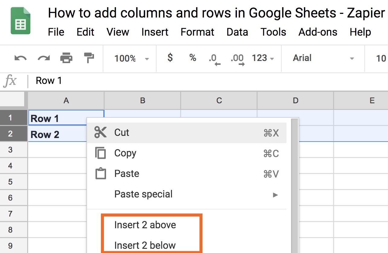
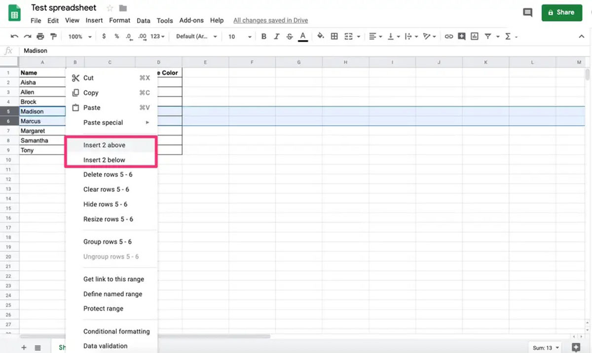
1. Move your cursor to the row you want to freeze: Look for the row number on the left-hand side of your sheet. If you want to freeze a single row, simply click on the row number to select it. If you need to freeze multiple rows, click and drag your cursor to select the desired rows.
2. Select consecutive rows: To select consecutive rows, click on the first row number, hold down the Shift key on your keyboard, and then click on the last row number. This will highlight all the rows in between.
3. Select non-consecutive rows: To select non-consecutive rows, hold down the Ctrl (or Command) key on your keyboard while clicking on the individual row numbers. This will highlight each selected row separately.

By selecting the specific row(s) you want to freeze, you’re telling Google Sheets to keep those rows visible at the top of the sheet, even as you scroll through the rest of your data. This ensures that important headers or information remains accessible and visible no matter where you are in your sheet.

Remember, freezing rows in Google Sheets can help improve your efficiency and overall user experience, especially when working with large datasets or complex spreadsheets. It’s a powerful feature that enables you to focus on the data that matters most without losing track of essential information.

Now that you’ve selected the row(s) you want to freeze, let’s move on to the next step and actually freeze the row(s).

Step 3: Freeze the Row

After selecting the row(s) you want to freeze in Google Sheets, it’s time to apply the freeze command and make sure that these rows remain visible while scrolling. Here’s how you can freeze the row:

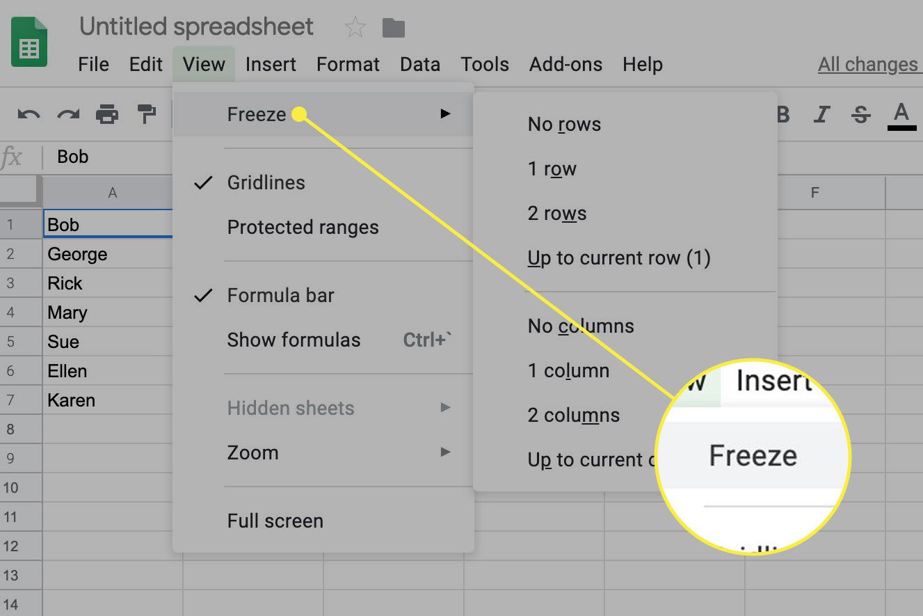
1. Navigate to the “View” menu: Look at the top of your Google Sheets interface and locate the “View” menu. Click on it to reveal a drop-down menu with various options.
2. Select the “Freeze” option: From the drop-down menu, hover your cursor over the “Freeze” option. This will open a sub-menu with different freezing options.
3. Select the number of rows to freeze: In the sub-menu, you will find options to freeze different numbers of rows. If you selected a single row, choose “1 row” to freeze only that row. If you selected multiple rows, select the corresponding number of rows to freeze.

By applying the freeze command, Google Sheets will lock the selected row(s) at the top of your sheet, allowing you to easily scroll through the rest of your data while keeping the important information in view.

It’s important to note that the freeze command is a toggle, meaning you can unfreeze the row(s) later if needed. To unfreeze rows, you can simply go back to the “View” menu, select “Freeze,” and then choose the “No rows” option.

Freezing rows is a powerful feature in Google Sheets that can save you time and effort. It ensures that essential information, such as headers or labels, remains visible and easily accessible, even as you navigate through large sheets.

Now that you’ve successfully frozen the row(s) in Google Sheets, let’s move on to the next step and learn how to adjust the frozen row to fit your needs.

Step 4: Adjust the Frozen Row

Once you have frozen a row in Google Sheets, you may want to make some adjustments to ensure optimal visibility and readability. Here are a few ways you can customize and adjust the appearance of the frozen row:

1. Resize the frozen row: To change the height of the frozen row, hover your cursor over the line below the frozen row until it changes to a resize cursor. Click and drag the line up or down to adjust the height to your desired size.
2. Set a specific row height: Alternatively, you can right-click on the row number of the frozen row and select “Row height” from the context menu. In the dialog that appears, enter a specific row height value, and click “OK” to apply the changes.
3. Format the frozen row: You can also apply formatting options to the frozen row, such as changing the font style, font color, background color, or adding borders. Simply select the cells within the frozen row and apply the desired formatting options from the toolbar or the Format menu.

By adjusting the frozen row to your preferences, you can ensure that the information remains clear and legible as you navigate through your sheet. This can be especially helpful when working with complex datasets or when presenting your sheet to others.

It’s worth noting that the adjustments made to the frozen row will apply to the entire row, including the non-frozen part. This ensures a consistent look and feel throughout your sheet, making it easier to interpret and work with your data.

Now that you know how to adjust the frozen row, you have complete control over its appearance and can fine-tune it based on your specific needs.

With the frozen row in place and customized to your liking, you can seamlessly work with your data in Google Sheets, improving both your productivity and the overall user experience.

Now let’s move on to some additional tips and tricks that can further enhance your workflow in Google Sheets.

Additional Tips and Tricks

Now that you have mastered the basic steps of freezing rows in Google Sheets, let’s explore some additional tips and tricks to enhance your experience and make the most out of this powerful spreadsheet tool:

1. Freezing multiple rows: As mentioned earlier, you can freeze multiple rows by selecting them before applying the freeze command. This can be useful when you have more than one header row or when you want to keep multiple rows of important information visible at all times.
2. Using the “Freeze” shortcut: Instead of navigating through the “View” menu, you can use a shortcut to freeze rows. Simply highlight the desired row(s) and press the shortcut keys: Ctrl + Alt + Shift + 1 (Windows) or Cmd + Option + Shift + 1 (Mac). Customize the number “1” to freeze the respectively selected number of rows.
3. Combining freezing rows and columns: In addition to freezing rows, you can also freeze columns in Google Sheets. This allows you to keep specific columns fixed on the left side of the sheet while scrolling horizontally. To freeze columns, simply select the desired column(s) and navigate to the “View” menu, then choose “Freeze” and “1 column” (or the number of columns you selected).
4. Unfreezing rows or columns: If you need to unfreeze rows or columns, simply go back to the “View” menu, select “Freeze,” and choose the “No rows” or “No columns” option, depending on what you want to unfreeze.
5. Experiment with different row heights: Play around with different row heights in your frozen row to find the optimal size for your content. This can help ensure that the frozen row takes up just the right amount of space without obstructing the rest of your sheet.
6. Regularly adjust frozen rows: As you work with your sheet, you might find that the content in your frozen row changes or expands. It’s a good practice to regularly review and adjust the frozen row to accommodate any modifications and ensure that all vital information remains visible.

By utilizing these tips and tricks, you can further customize and optimize your frozen rows in Google Sheets, making your data management and analysis experience even smoother and more efficient.

Now that you’re armed with these additional tips, feel free to explore and experiment in Google Sheets to discover even more ways to enhance your workflow and maximize your productivity.

Conclusion

Freezing rows in Google Sheets is a valuable technique that allows you to keep important information visible while scrolling through large datasets. By following the simple steps outlined in this article, you can effortlessly freeze rows and enhance your productivity.

Through the process of freezing a row, you can improve data analysis, ease navigation, promote efficient collaboration, and create presentation-ready sheets. Whether you’re a student, professional, or business owner, the ability to freeze rows in Google Sheets can significantly streamline your workflow and make working with spreadsheets a breeze.

By adjusting the frozen row and utilizing additional tips and tricks, such as freezing multiple rows, using shortcuts, combining freezing rows and columns, and regularly adjusting frozen rows, you can further enhance your experience and customize it to suit your specific needs.

Now that you have a solid understanding of how to freeze rows in Google Sheets, it’s time to apply this knowledge to your own sheets and simplify your data management processes. Remember to practice and explore different features and functionalities in Google Sheets to uncover even more possibilities.

So go ahead, freeze those rows, improve your data analysis, and optimize your workflow in Google Sheets. The world of organized and efficient data management awaits!