How To Add A Header In Google Sheets

Why Should You Add a Header in Google Sheets

Headers play a vital role in organizing and optimizing your data in Google Sheets. They provide a clear and concise way to identify the contents of each column, making it easier to navigate and understand the data in your spreadsheet.

Adding a header can significantly enhance the readability and usability of your Google Sheet. Here are a few reasons why you should consider adding a header:

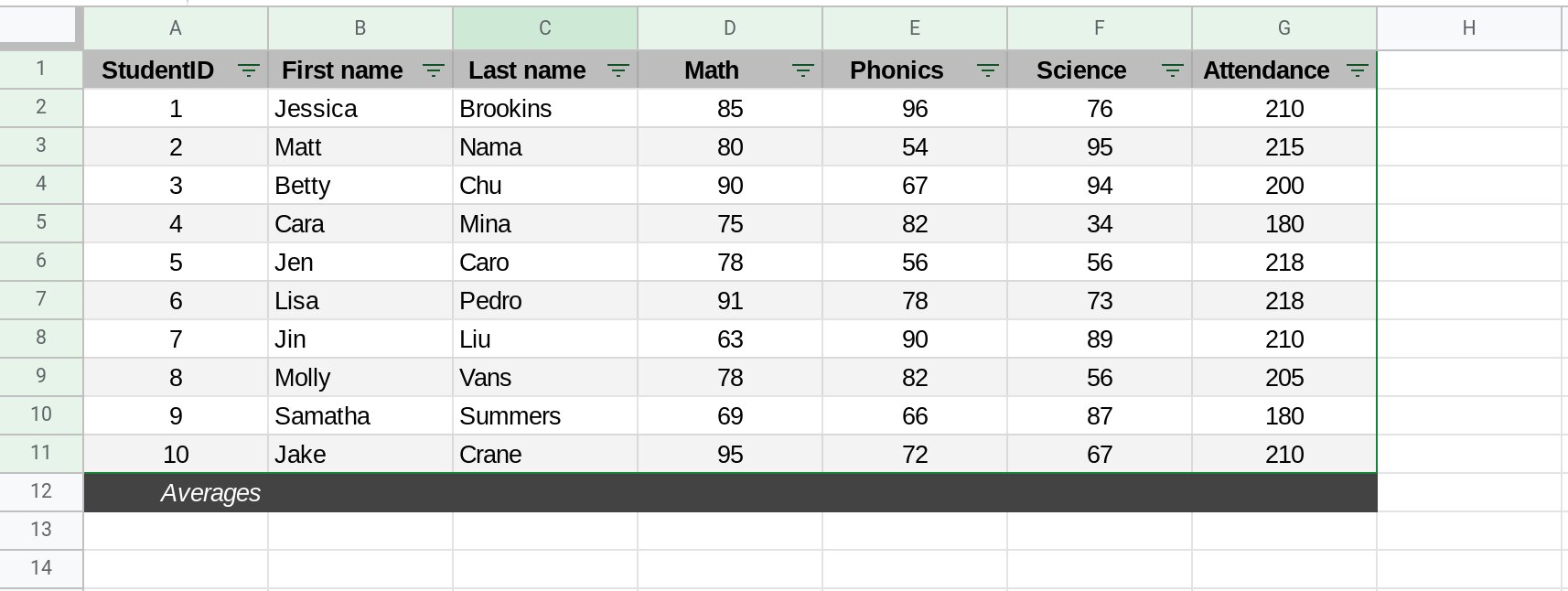
• Improved Data Interpretation: Headers provide a brief description of the data contained in each column. By adding clear, descriptive headers, you can quickly understand the type of information each column represents, making it easier to interpret and analyze the data.
• Efficient Sorting and Filtering: Headers allow you to sort and filter your data with ease. By identifying the headers for each column, you can arrange the data in ascending or descending order, facilitating the identification of trends and patterns. Filtering data becomes more straightforward as well, as you can specify the criteria based on the headers.
• Enhanced Collaboration: When collaborating with others on a Google Sheet, headers provide a consistent format for organizing and discussing data. By using descriptive headers, you can ensure that everyone understands the purpose of each column, reducing confusion and enhancing collaboration.
• Easy Navigation: Headers act as visual cues, allowing you to quickly locate the relevant information in a large spreadsheet. Instead of manually scrolling through rows, you can quickly jump to a specific column by referring to the headers, saving you time and effort.
• Improved Data Validation: Headers can also be used for data validation purposes. You can specify the type of data that should be entered in each column and include any validation rules to ensure data consistency and accuracy.

By adding a header in Google Sheets, you not only enhance the overall appearance of your spreadsheet but also improve data interpretation, sorting, filtering, collaboration, navigation, and validation. The benefits of incorporating headers are numerous and can greatly improve the efficiency and usability of your Google Sheets.

Step 1: Open Google Sheets

Before you can add a header in Google Sheets, you need to open the Google Sheets application. Follow these simple steps to access your Google Sheets:

1. Open your web browser and go to https://www.google.com/sheets/about/.
2. Sign in to your Google account. If you do not have an account, you can create one by clicking on the “Create account” button.
3. Once signed in, you will be directed to the Google Sheets homepage. Here, you can create a new spreadsheet or access any existing spreadsheets.
4. If you want to create a new spreadsheet, click on the “Blank” option to start with a fresh sheet. If you have an existing spreadsheet where you want to add a header, locate and click on the relevant sheet to open it.

Once you have opened Google Sheets and selected the desired spreadsheet, you are ready to proceed to the next step of adding a header.

It’s important to note that Google Sheets is a powerful and convenient web-based application that allows you to create, edit, and collaborate on spreadsheets. With its user-friendly interface and a range of features, it has become a popular choice for individuals and businesses alike.

By following this step, you have successfully accessed Google Sheets and are now ready to add a header to your spreadsheet. Keep reading to discover the next steps for adding a header in Google Sheets.

Step 2: Select a Cell Range for the Header

To add a header in Google Sheets, you first need to select the cell range where you want the header to appear. Follow these steps to choose the appropriate cell range:

1. Open your desired spreadsheet in Google Sheets.
2. Locate the row where you want to add the header. Typically, headers are added in the first row of the spreadsheet, but you can choose any row that suits your needs.
3. Click on the cell in the first column of the chosen row. This cell will become the starting point of your header.
4. Drag your cursor or use the Shift key to select the desired number of cells you want to include in your header. For example, if you want a header spanning three columns, select three cells in sequence.
5. Release the mouse button or the Shift key once you have selected the desired cell range. The selected cells will be highlighted, indicating the range for your header.

It’s essential to choose the appropriate cell range for your header to ensure that it covers the necessary columns and data. You can select as few or as many cells as needed, depending on the number of columns you want to include in your header.

If you want to include additional rows or modify the cell range later, you can easily adjust the selection by clicking and dragging the cells or using keyboard shortcuts.

By following these steps, you have successfully selected the cell range for your header in Google Sheets. Now it’s time to move on to the next step and add the header to your selected cell range.

Step 3: Click on the “Insert” Menu

After selecting the cell range for your header in Google Sheets, it’s time to add the header itself. To do this, you will need to navigate to the “Insert” menu. Follow these steps:

1. Make sure you have the selected cell range for the header in your spreadsheet.
2. Look at the top navigation menu in Google Sheets. Locate and click on the “Insert” option. This will open a drop-down menu with various options for inserting different elements into your spreadsheet.
3. In the “Insert” menu, you will find a range of options such as “Chart,” “Function,” “Drawing,” and more. To continue adding a header, choose the “Rows above” or “Rows below” option, depending on where you want your header to appear.
4. If you select “Rows above,” Google Sheets will insert a new row above the selected cell range. If you choose “Rows below,” the application will insert a row below the selected cell range. This new row will serve as the dedicated space for your header.

The “Insert” menu in Google Sheets provides a convenient way to add additional rows or elements to your spreadsheet, including headers. By selecting the appropriate option in the menu, you can seamlessly integrate the header into your spreadsheet layout.

Once you have clicked on the “Insert” menu and chosen either “Rows above” or “Rows below,” you are ready to move on to the next step and customize your header to suit your needs.

Step 4: Choose “Rows Above” or “Rows Below”

After accessing the “Insert” menu in Google Sheets, the next step is to determine whether you want to add the header rows above or below the selected cell range. Follow these steps to make your choice:

1. Ensure that you have opened the “Insert” menu in Google Sheets and have selected the cell range for your header.
2. In the “Insert” menu, look for the options labeled “Rows above” and “Rows below.” These options define the placement of the new row that will serve as your header.
3. If you want to have the header appear above the selected cell range, choose the “Rows above” option. Google Sheets will insert a new row above the selected range, effectively creating space for you to add your header.
4. If you prefer the header to appear below the selected cell range, select the “Rows below” option. Google Sheets will insert a new row below the selected range where you can add your header.

Choosing between “Rows above” and “Rows below” depends on your preferred visual layout and the logical positioning of the header within your spreadsheet. Consider the organization and flow of your data to determine the most appropriate placement for your header.

By making this selection in the “Insert” menu, you are one step closer to adding and customizing your header in Google Sheets. Remember to consider the overall design and readability of your spreadsheet as you move forward with the next steps.

Step 5: Customize the Header

After inserting the new row for your header in Google Sheets, it’s time to customize and personalize it according to your preferences. Follow these steps to tailor your header:

1. Locate the newly inserted row that serves as your header. This row will be directly above or below the selected cell range.
2. Click on the cells within the header row to enter the desired text for each column. You can use descriptive labels, abbreviations, or any other text that clearly represents the data in the corresponding column.
3. Adjust the width of each cell in the header row if needed. To do this, hover your cursor over the gridline between two columns until it changes to a double-sided arrow. Click and drag the gridline to expand or shrink the width of the cell as required.
4. Select and apply formatting options to enhance the appearance of your header. You can utilize the various formatting tools available in Google Sheets, such as font style, font size, bold or italic text, cell background color, and more.
5. Consider merging cells in the header row if you have multiple columns that require a broader header. To merge cells, click and drag to select the cells you want to merge, right-click, and choose the “Merge cells” option from the context menu.

Customizing the header allows you to make it visually appealing and easy to read. By using clear and concise labels, adjusting cell widths, applying formatting options, and merging cells when necessary, you can create a header that effectively organizes and represents your data.

Remember, customization options in Google Sheets are abundant, giving you the flexibility to make your header standout. But, it’s important to strike a balance between creativity and readability to ensure that your header remains easy to understand and navigate.

Once you have tailored your header to your liking, it’s time to move on to the next step and format the header text to make it even more visually appealing.

Step 6: Format the Header Text

Formatting the header text in Google Sheets can help improve its readability and make it visually appealing. Follow these steps to format the header text according to your preferences:

1. Select the cells containing the header text that you want to format. This could be the entire header row or specific cells within it.
2. In the toolbar at the top of the Google Sheets interface, you will find various formatting options. These include font style, font size, font color, bold, italic, underline, and more.
3. Click on the desired formatting option to apply it to the selected header text. For example, to make the text bold, click on the “B” icon in the toolbar. Similarly, you can click on the “I” icon to make the text italic or the “U” icon to underline the text.
4. If you want to change the font style or size, click on the corresponding drop-down menus in the toolbar and select your preferred options.
5. For additional formatting options, such as text alignment, cell background color, or number formatting, you can utilize the “Format” menu in the toolbar or right-click on the selected cells and access the context menu.

Formatting the header text allows you to make it more visually appealing, emphasize important information, and create a consistent and professional look for your spreadsheet. Consider using a font style and size that is easy to read, and utilize formatting options that enhance the clarity and organization of the data in your header.

Remember, while formatting the header text can make it visually appealing, it’s important to avoid excessive or inconsistent formatting that may hinder the readability of the header. Maintain a balance between aesthetics and functionality to ensure that your header remains clear and easy to understand.

Once you have formatted the header text to your satisfaction, you can proceed to the next step and apply any additional formatting to enhance your Google Sheet.

Step 7: Apply Any Additional Formatting

In addition to formatting the header text, you can apply various other formatting options to enhance the overall appearance and functionality of your Google Sheet. Follow these steps to apply any additional formatting:

1. Select the cells in your Google Sheet that you want to format. This could be the header cells, data cells, or other relevant sections of your spreadsheet.
2. Utilize the formatting tools available in the toolbar or the “Format” menu to make adjustments. Some common formatting options include changing cell background color, modifying text alignment, adjusting borders, and applying conditional formatting rules.
3. If you want to customize the appearance of your entire spreadsheet, you can access the “Format” menu and explore options such as freeze rows or columns, add borders, adjust column width or row height, and more.
4. Consider applying conditional formatting rules to highlight specific data based on predefined criteria. This can be useful for identifying trends, outliers, or important information in your spreadsheet.
5. Continue experimenting with different formatting options until you achieve a visually pleasing and organized layout for your Google Sheet.

Applying additional formatting to your Google Sheet allows you to tailor it to your specific needs and improve visual clarity. Remember to strike a balance between aesthetics and functionality, keeping the overall readability and usability of your sheet in mind.

It’s important to note that formatting options in Google Sheets are extensive and can help you create a professional and well-structured spreadsheet. However, it’s advisable to avoid excessive formatting that might overwhelm the data and make it difficult to comprehend.

Once you have applied any additional formatting to your Google Sheet, you can proceed to the final step: saving and sharing your spreadsheet.

Step 8: Save and Share Your Google Sheet

After adding headers, customizing the layout, and formatting your Google Sheet, it’s time to save your work and share it with others. Follow these steps to save and share your Google Sheet:

1. Click on the “File” menu located at the top left corner of the Google Sheets interface.
2. In the drop-down menu, select the “Save” option to save your changes. Google Sheets automatically saves your sheet as you work, but it’s always a good practice to manually save to ensure your updates are applied.
3. If you want to rename your sheet, click on the “File” menu again and select the “Rename” option. Enter a new name for your sheet and click “Save” to confirm the changes.
4. To share your Google Sheet with others, click on the blue “Share” button located on the top right corner of the screen. A sharing settings window will appear, allowing you to specify who can access and edit the sheet.
5. Enter the email addresses of the individuals you want to share the sheet with. You can also set their permissions, choosing whether they can only view, comment, or edit the sheet.
6. After setting the sharing permissions, click on the “Send” button. This will send an email invitation to the specified recipients, allowing them to access and collaborate on the Google Sheet.

By saving and sharing your Google Sheet, you ensure that your hard work is securely stored and accessible to the right people. Collaboration and sharing are integral features of Google Sheets, allowing you to work efficiently and effectively with others on your spreadsheet.

Remember to regularly save your Google Sheet as you make changes to avoid losing any progress. Additionally, as you collaborate with others, make sure to communicate and coordinate effectively to maintain data integrity and achieve your goals.

Congratulations! You have successfully saved and shared your Google Sheet, allowing others to benefit from the organized layout and visually appealing header you have created.