How Do You Alphabetize In Google Sheets

Introduction

Alphabetizing data in Google Sheets is a useful feature that allows you to arrange your information in a logical and organized manner. Whether you’re working with a single column or multiple columns, the ability to sort data alphabetically can simplify data management, improve readability, and make it easier to find specific information.

Google Sheets provides several options for alphabetizing your data, including sorting a single column, sorting multiple columns simultaneously, and sorting by custom order. These features give you the flexibility to arrange your data in a way that best suits your needs and preferences.

In this article, we will explore various methods to alphabetize data in Google Sheets. We will cover how to alphabetize a single column, how to alphabetize multiple columns, and even how to sort a range of cells. Additionally, we will discuss how to ignore articles and prepositions when sorting, how to sort by custom order, and how to sort in ascending or descending order.

Furthermore, we will delve into sorting by multiple criteria, allowing you to sort your data based on multiple factors simultaneously. We will also touch upon the importance of knowing how to undo a sort, in case you make a mistake or need to revert to the original order.

By the end of this article, you will have a comprehensive understanding of how to alphabetize data in Google Sheets efficiently and effectively, enabling you to organize your data in a way that best serves your needs.

Alphabetizing a Single Column

When you need to alphabetize a single column in Google Sheets, follow these simple steps:

Select the column by clicking on the header. The entire column will now be highlighted.
Next, go to the “Data” menu and select “Sort sheet by column A” (or the appropriate column letter). Alternatively, you can use the shortcut Ctrl + Shift + Sort Range.
A small popup window will appear, allowing you to customize the sort options. By default, the column will be sorted in ascending order. You can also choose to sort in descending order by ticking the corresponding option.
Once you’ve set your preferences, click on the “Sort” button, and Google Sheets will alphabetize the data in the selected column.

It’s important to note that when alphabetizing a single column, the sort will affect only the selected column. The rest of the data in the sheet will remain unaffected.

Additionally, if your column contains data with numbers or special characters, Google Sheets will prioritize the alphabetical order and place these entries accordingly. For example, if you have names like “John”, “Mary”, and “123ABC” in a column, Google Sheets will sort them as “123ABC”, “John”, and “Mary”.

This method works well for organizing data in a single column and is especially useful for sorting lists, contacts, or any data that needs to be arranged alphabetically based on a specific criterion.

By following these instructions, you’ll be able to alphabetize a single column in Google Sheets quickly and efficiently. This feature can make it easier to find specific entries and ensure that your data is organized in a logical and accessible manner.

Alphabetizing Multiple Columns

In addition to alphabetizing a single column, Google Sheets also allows you to alphabetize multiple columns simultaneously. This feature is particularly useful when you want to maintain the relationship between different sets of data.

To alphabetize multiple columns in Google Sheets, follow these steps:

Select the range of columns you want to alphabetize. You can do this by clicking and dragging your cursor across the column headers.
Once the columns are selected, go to the “Data” menu and choose “Sort range”. Alternatively, you can use the shortcut Ctrl + Shift + Sort Range.
In the popup window that appears, you have the option to specify the primary column for sorting. This is the column that will be used as the primary criterion for alphabetizing the data. Select the appropriate column from the “Sort by” dropdown menu.
By default, the sort order is set to ascending. If you prefer descending order, you can check the corresponding checkbox.
After setting your preferences, click on the “Sort” button, and Google Sheets will alphabetize the data in the selected columns based on the primary column you specified.

This method allows you to maintain the integrity of your data across multiple columns while arranging them alphabetically. It’s particularly useful when you have corresponding information in different columns, such as names and contact details. Alphabetizing multiple columns together ensures that the data remains synchronized.

Keep in mind that when alphabetizing multiple columns, Google Sheets considers the primary column as the main sorting criterion. If there are duplicate entries in the primary column, Google Sheets will then consider the secondary column to determine the order.

By following these steps, you can easily alphabetize multiple columns in Google Sheets, enabling you to organize your data cohesively and maintain the relationship between different sets of information.

Sorting a Range of Cells

In addition to sorting individual columns, Google Sheets also provides the functionality to sort a range of cells. This feature is particularly helpful when you want to sort a specific section of your sheet or when you have data that spans across multiple columns and rows.

To sort a range of cells in Google Sheets, follow these steps:

Select the range of cells you want to sort. You can do this by clicking and dragging your cursor across the desired cells.
Go to the “Data” menu and select “Sort range”. Alternatively, you can use the shortcut Ctrl + Shift + Sort Range.
In the popup window, Google Sheets will automatically detect the selected range of cells. If the selection spans multiple columns, you can choose the primary column for sorting by selecting it from the “Sort by” dropdown menu.
You can set the sort order to ascending or descending by checking the corresponding checkbox.
Once you’ve chosen your sort preferences, click on the “Sort” button, and Google Sheets will rearrange the selected range of cells based on the specified criteria.

This method allows you to sort a specific range of cells, regardless of whether they are contiguous or scattered throughout your sheet. It provides greater flexibility in organizing your data and allows you to focus on specific subsets of information when sorting.

When sorting a range of cells, Google Sheets follows the same rules as when sorting single columns or multiple columns. This means that if your range contains both text and numeric data, Google Sheets will prioritize the alphabetical order and place these entries accordingly.

By utilizing the range sorting feature in Google Sheets, you can easily sort a specific section of your sheet or sort data that spans across multiple columns and rows. This gives you greater control over how your data is organized and enhances the readability and accessibility of your sheet.

Ignoring Articles and Prepositions

When alphabetizing data, it is common to ignore certain words, such as articles (e.g., “a,” “an,” “the”) and prepositions (e.g., “in,” “on,” “at”). Ignoring these words helps to focus on the core content and avoids unnecessary clutter in the sorted list.

In Google Sheets, you can customize the sorting process to ignore articles and prepositions by following these steps:

Select the column or range of cells you want to sort. You can do this by clicking and dragging your cursor across the desired cells.
Go to the “Data” menu and choose “Sort sheet by column A” (or the appropriate column letter). Alternatively, you can use the shortcut Ctrl + Shift + Sort Range.
In the popup window that appears, click on the “Data has header row” checkbox if your data includes a header row that you want to exclude from the sorting process.
Next, check the “Sort by” box and select “Custom sort order” from the dropdown menu.
A new section will appear where you can define your custom sort order. Here, you can create a list of words to ignore, such as articles and prepositions, by entering them in the “Custom order” box, separated by commas.
After specifying your custom sort order, click on the “Sort” button to alphabetize the data while excluding the designated words.

By enabling the option to ignore articles and prepositions, Google Sheets will sort the data without considering these words. This can provide a cleaner and more focused sorting result, making it easier to locate specific entries in the list.

The ability to ignore articles and prepositions is particularly beneficial when sorting data that contains titles, names, or phrases where these words do not carry significant meaning or sorting relevance.

By utilizing the custom sort order feature in Google Sheets, you can easily alphabetize your data while excluding articles and prepositions. This helps you maintain a clean and relevant sorted list that prioritizes the main content.

Sorting by Custom Order

In some cases, you may want to sort your data in a specific order that does not follow alphabetical or numerical patterns. Google Sheets allows you to customize the sort order by defining your own custom order criteria.

To sort data by custom order in Google Sheets, follow these steps:

Select the column or range of cells you want to sort. You can do this by clicking and dragging your cursor across the desired cells.
Go to the “Data” menu and choose “Sort sheet by column A” (or the appropriate column letter). Alternatively, you can use the shortcut Ctrl + Shift + Sort Range.
In the popup window that appears, click on the “Data has header row” checkbox if your data includes a header row that you want to exclude from the sorting process.
Next, check the “Sort by” box and select “Custom sort order” from the dropdown menu.
A new section will appear where you can define your custom sort order. Enter your desired order criteria by listing the values in the “Custom order” box, separated by commas. The entered values should match the ones in the column exactly.
After specifying your custom sort order, click on the “Sort” button to sort the data according to your specified criteria.

By using the custom sort order feature, you have the flexibility to define the desired order for your data. This is particularly beneficial when you have non-alphabetical or non-numeric values that need to be sorted according to a specific custom order, such as priority levels, stages, or categories.

Sorting by custom order allows you to arrange your data in a way that aligns with your unique requirements. It helps you prioritize specific values or categories and ensures that your data is organized according to your specific criteria.

By following these steps, you can easily sort your data by custom order in Google Sheets, giving you the freedom to arrange your data according to the desired criteria and enhancing the clarity and usability of your spreadsheet.

Sorting in Ascending or Descending Order

When sorting data in Google Sheets, you have the flexibility to arrange it in either ascending or descending order. Sorting in ascending order means that the values will be arranged from smallest to largest or from A to Z, while sorting in descending order means the values will be arranged from largest to smallest or from Z to A.

To sort data in ascending or descending order in Google Sheets, follow these steps:

Select the column or range of cells you want to sort. You can do this by clicking and dragging your cursor across the desired cells.
Go to the “Data” menu and choose “Sort sheet by column A” (or the appropriate column letter). Alternatively, you can use the shortcut Ctrl + Shift + Sort Range.
In the popup window that appears, click on the “Data has header row” checkbox if your data includes a header row that you want to exclude from the sorting process.
By default, Google Sheets sorts data in ascending order. If you want to sort in descending order, check the “Z → A” option.
After selecting your desired sorting order, click on the “Sort” button to rearrange the data according to the chosen criteria.

Sorting in ascending or descending order provides you with control over the arrangement of your data based on its value or alphabetical order. It allows you to prioritize and highlight the most significant or prominent values in your dataset, making it easier to identify trends or find specific entries.

It’s important to note that when sorting in descending order, the numeric values will be arranged from largest to smallest, and alphabetically, the values will be arranged from Z to A. This can be particularly useful when you want to identify outliers, high or low values, or find the last entry in a sorted list.

By utilizing the ascending and descending sorting options in Google Sheets, you can easily rearrange your data in the desired order, improving its readability and enabling a better understanding of your dataset.

Sorting by Multiple Criteria

Sorting data based on a single criterion is useful, but there are situations where you may want to sort your data using multiple criteria. Google Sheets allows you to sort your data by multiple criteria, giving you more control over the arrangement and organization of your data.

To sort data by multiple criteria in Google Sheets, follow these steps:

Select the range of cells you want to sort. This can be a single column or multiple columns.
Go to the “Data” menu and choose “Sort range” or use the shortcut Ctrl + Shift + Sort Range.
In the popup window that appears, you can specify multiple sort columns by clicking on the “Add another sort column” button.
For each sort column, choose the column you want to sort by and select the sort order (ascending or descending).
Arrange the sort columns in the desired order by using the arrows next to each sort column.
Click on the “Sort” button to sort the data based on the multiple criteria you set.

By sorting data with multiple criteria, you can refine the order of your data based on multiple factors. This can be particularly useful when you have complex datasets with multiple attributes that you want to prioritize in the sorting process.

When sorting by multiple criteria, Google Sheets first sorts the data based on the primary criterion you set. If there are ties in the primary criterion, it then considers the secondary criterion, and so on. This allows you to establish a hierarchy of sorting criteria.

Sorting data by multiple criteria provides a more nuanced and tailored approach to arranging your data. It allows you to consider various factors simultaneously and ensures that your data is organized according to multiple dimensions or priorities.

By following these steps, you can easily sort your data by multiple criteria in Google Sheets, giving you greater control over the arrangement and structure of your data and facilitating a deeper understanding of the relationships within your dataset.

Undoing Sort

Sorting data in Google Sheets can be a powerful tool for organizing and analyzing your information. However, there may be instances when you want to revert back to the original order or undo a previous sort operation. Google Sheets provides a straightforward way to undo a sort, allowing you to restore your data to its original arrangement.

To undo a sort in Google Sheets, follow these steps:

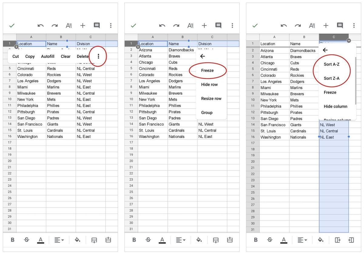
Click on the arrow at the top-left corner of your data range. This selects the entire sheet.
Go to the “Data” menu and choose “Sort range” or use the shortcut Ctrl + Shift + Sort Range.
In the popup window that appears, you will notice that the sort criteria are displayed for each column. To undo the sort, simply click on the “x” button next to each column’s sort criteria. This will remove the sort criteria for that specific column.
Once you have removed the sort criteria for all columns, click on the “Sort” button to restore your data to its original order.

By undoing a sort, your data will return to the original arrangement before any sorting was applied. This can be helpful when you realize that the sorting doesn’t produce the desired outcome, or if you simply need to revert back to the original unsorted version of your data.

It’s essential to note that undoing a sort will remove all the sorting criteria applied to your data range. Therefore, it’s important to double-check if you want to undo the sort for the entire sheet or only for specific columns.

By following these steps, you can easily undo a sort operation in Google Sheets, restoring your data to its original order and giving you the flexibility to explore different sorting options without permanently altering your data.

Conclusion

Alphabetizing data in Google Sheets is an essential skill that allows you to organize information in a logical and accessible manner. Whether you need to sort a single column, multiple columns, a range of cells, or even ignore certain words or sort by custom order, Google Sheets provides a range of features to help you achieve your desired sorting results.

By alphabetizing data, you can enhance readability, easily find specific entries, and gain insights from your information. The ability to sort in ascending or descending order, sort by multiple criteria, and undo a sort allows you to have precise control over the arrangement of your data.

Remember to use markdown formatting, including headings and bulleted lists, to present the information in an organized and engaging manner. Additionally, infusing creativity, human-like language, and natural sentence structures into your writing will captivate readers and make your content more enjoyable to read.

With the knowledge and skills gained from this article, you can confidently sort and alphabetize your data in Google Sheets, optimizing your data management and analysis capabilities.