How To Create Filters In Google Sheets

Introduction

Welcome to this tutorial on how to create filters in Google Sheets. Filters are a powerful tool that allow you to manipulate and analyze data in your spreadsheets. Whether you want to sort data, extract specific information, or apply custom criteria to narrow down your results, filters can help you achieve these tasks efficiently.

Filters in Google Sheets enable you to view only the data that meets certain criteria, hiding the rest of the rows that don’t match. This can be incredibly useful when dealing with large datasets or when you need to focus on specific information.

In this tutorial, we will explore different ways to utilize filters in Google Sheets. We will cover how to set up your data, use the filter function, apply filters based on various criteria, and sort the filtered data. Additionally, we will learn how to clear filters when they are no longer needed.

By the end of this tutorial, you will have a thorough understanding of how to efficiently use filters in Google Sheets to organize your data and extract valuable insights. So, let’s dive in and get started!

Setting Up Your Data

Before you can start applying filters in Google Sheets, it’s important to ensure that your data is properly organized. To set up your data for filtering, follow these steps:

1. Open a new or existing Google Sheet: Launch Google Sheets and create a new spreadsheet or open an existing one in which you want to apply filters.
2. Create headers: In the first row of your spreadsheet, create headers for each column. These headers should clearly indicate the type of data in each column. For example, if you have a dataset of sales records, you might have headers such as “Date,” “Product,” “Quantity,” and “Price.”
3. Enter your data: Starting from the second row, enter your data below the corresponding headers. Make sure each entry is placed in the appropriate column. Fill in all the necessary information for your dataset.
4. Format your data: Apply any formatting options required to make your data more visually appealing and easier to read. This may include setting text styles, adjusting column widths, or applying number formatting for numerical data.

Once you have set up your data in this manner, you are ready to start utilizing filters in Google Sheets. Having well-organized and properly formatted data will make it easier to apply filters effectively and extract the information you need.

Using the Filter Function

In Google Sheets, the Filter function is a powerful tool that allows you to quickly and easily apply filters to your data. This function enables you to specify criteria for filtering and displays only the rows that meet those criteria. Follow these steps to use the Filter function:

1. Select the data: Click on the cell that contains the header of your data range. Then, drag the mouse to select the entire range of data you want to apply the filter to.
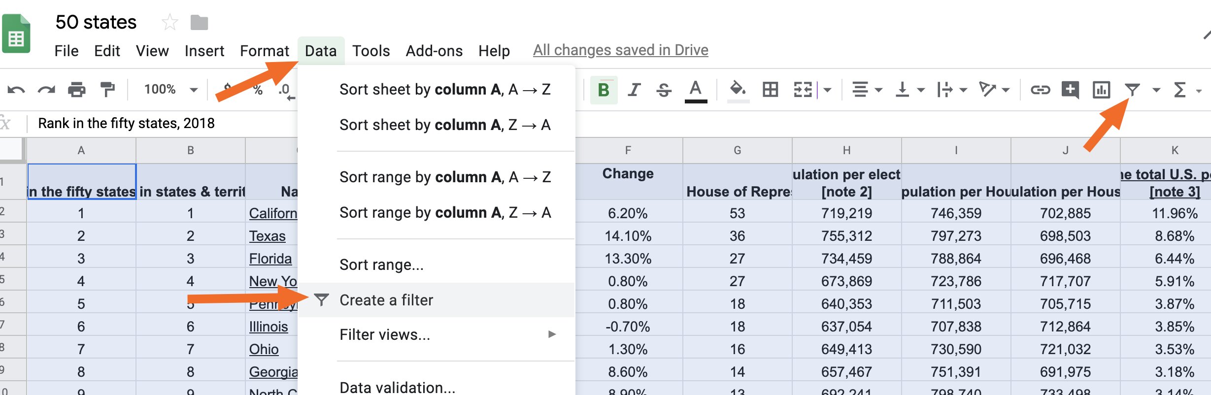
2. Open the Filters menu: Go to the “Data” menu and click on “Filter.”
3. Apply the filter: In the header row, you will notice small arrows appear next to each column. Click on the arrow of the column you want to filter.

Once you click on the arrow, a drop-down menu will appear with various options. You can choose from a list of unique values in that column, sort the column in ascending or descending order, or even create a custom filter.

If you want to apply a custom filter, choose the “Filter by condition” option from the drop-down menu. This allows you to specify specific conditions based on the values in the selected column. For example, you can filter to show only values greater than a certain number or within a certain range.

After selecting your desired filter option, Google Sheets will hide the rows that don’t meet the specified criteria. You can apply filters to multiple columns simultaneously to refine your results further.

To remove the filters, go back to the “Data” menu and click on “Turn off filters.” This will show all the hidden rows and revert your spreadsheet to its original state without any filters applied.

The Filter function in Google Sheets provides an easy and flexible way to analyze data by narrowing down the results based on specific criteria. It allows you to focus on the information that is most relevant to your needs and makes data analysis more efficient and streamlined.

Applying Filters

Once you have set up your data and understood how to use the Filter function in Google Sheets, you can start applying filters to narrow down your results. Applying filters allows you to focus on specific data points that meet certain criteria. Here’s how to apply filters:

1. Select the data range: Click on any cell within your data range or select the entire range you want to filter.
2. Open the Filters menu: Go to the “Data” menu and click on “Filter.”
3. Apply filters: Once the Filters menu is open, you will notice arrows next to each column header. Click on the arrow of the column you want to filter.

A drop-down menu will appear, displaying various filter options depending on the data type in that column. You can choose from options like text contains, number greater than, date is before, and more. Select the option that best suits your filtering needs.

If you want to filter by multiple criteria, you can do so by adding additional filters to other columns. Google Sheets will show only the rows that meet all the specified criteria, successfully narrowing down your dataset.

You can also use the Filter function to filter by values that are not equal to a specific criterion. For example, if you want to filter out all the rows where the value in a column is not equal to a particular number, you can select the “Does not equal” option from the filter menu.

Remember, you can apply filters to all types of data, including text, numbers, and dates. This flexibility allows you to precisely refine your results and extract the information you need for analysis or reporting.

Once you have applied your filters, the rows that don’t meet the specified filter criteria will be hidden from view, making it easier to focus on the relevant data. To remove the filters, go back to the “Data” menu and click on “Turn off filters.” This will restore your spreadsheet to its original state without any filters applied.

Applying filters in Google Sheets is an efficient way to sift through large datasets and extract the desired information based on specific criteria. By utilizing the filtering capabilities, you can gain valuable insights from your data and make data-driven decisions with ease.

Filtering by Date

Filtering by date in Google Sheets allows you to extract specific data based on date ranges or specific dates. This can be particularly useful when working with datasets that include time-sensitive information or when you want to analyze data within a certain time frame. Here’s how to filter by date in Google Sheets:

1. Select the data range: Click on any cell within your data range or select the entire range that includes the date column you want to filter.
2. Open the Filters menu: Go to the “Data” menu and click on “Filter.”
3. Apply the date filter: Click on the filter arrow next to the date column header.
   • If you want to filter by a specific date, select the date value from the drop-down menu.
   • If you want to filter by a date range, choose the “Date range” option from the drop-down menu.

If you choose the “Date range” option, a sub-menu will appear, allowing you to specify the start and end dates of the range. Google Sheets will then display only the rows that fall within the selected date range.

Furthermore, you can also use the “Before” and “After” options to filter data based on dates before or after a specific date. This is helpful when you want to focus on data that occurred before or after a particular event.

Additionally, you can apply other filter options in combination with filtering by date to further refine your results. For example, you can filter data by date and another criteria, such as filtering by a specific product or a customer.

Remember, once you have applied the date filter, Google Sheets will only display the rows that meet your specified criteria. To remove the filter, go back to the “Data” menu and click on “Turn off filters.”

Filtering by date in Google Sheets allows you to extract specific information from your dataset based on time-sensitive data. Whether you need to analyze trends over a particular period or focus on specific dates, applying date filters can help you efficiently work with your data.

Filtering by Custom Criteria

When working with data in Google Sheets, you may often want to filter your dataset based on specific criteria that are not covered by the default filter options. The good news is that you can apply custom filters in Google Sheets, allowing you to define your own filtering conditions. Here’s how to filter by custom criteria:

1. Select the data range: Click on any cell within your data range or select the entire range that includes the column you want to filter by custom criteria.
2. Open the Filters menu: Go to the “Data” menu and click on “Filter.”
3. Apply the custom filter: Click on the filter arrow next to the column header you want to filter by custom criteria. In the drop-down menu, select the “Filter by condition” option.
4. Specify the filtering condition: In the dialog box that appears, you can create your custom filtering condition. Google Sheets provides various options to choose from, such as “Text contains,” “Number greater than,” “Date is before,” and many others. Select the option that matches your desired filtering condition.
5. Set the filtering value: Based on the condition you selected, you need to specify the value to be used for the filter. Enter the value in the text box provided.
6. Apply the custom filter: Click on the “OK” button to apply the custom filter. Google Sheets will hide the rows that don’t meet your specified condition, displaying only the rows that match your custom criteria.

By using custom filters, you have the flexibility to define your own unique criteria for filtering your data. You can use comparison operators, such as equals, not equals, greater than, less than, and more, to create specific conditions that suit your data analysis needs.

Remember, you can apply custom filters to multiple columns simultaneously to refine your results further. This allows you to create complex filtering conditions to extract specific information from your dataset.

To remove the custom filters, go back to the “Data” menu and click on “Turn off filters.” This will remove all the applied filters and display your spreadsheet without any filtering conditions.

Filtering by custom criteria in Google Sheets empowers you to filter your data based on unique conditions that match your specific analysis requirements. It provides you with the flexibility and control to extract the precise information you need from your dataset.

Applying Multiple Filters

Google Sheets allows you to apply multiple filters to your data, giving you the ability to refine your results and extract precise information that meets multiple criteria simultaneously. Applying multiple filters can help you analyze and organize your data more effectively. Here’s how to apply multiple filters in Google Sheets:

1. Select the data range: Click on any cell within your data range or select the entire range that includes the columns you want to filter.
2. Open the Filters menu: Go to the “Data” menu and click on “Filter.”
3. Apply the first filter: Click on the filter arrow of the column you want to apply the first filter to. Choose your filter criteria from the drop-down menu as we discussed earlier.
4. Apply additional filters: To add more filters, click on the filter arrows of the other columns where you want to apply filters. Choose your additional filter criteria for each column.

Google Sheets will apply all the specified filters simultaneously, showing only the rows that meet all the filtering criteria. This allows you to further narrow down your dataset to the exact information you need.

It’s important to note that when applying multiple filters, the filtering logic follows the “AND” condition. This means that for a row to be displayed, it must satisfy all the filtering conditions specified across different columns.

You can continue to add more filters to as many columns as needed, creating complex combinations of criteria for refining your data. This flexibility allows you to perform in-depth data analysis and extract valuable insights.

It’s worth mentioning that you can also apply both custom filters and predefined filter options simultaneously. This gives you even more control over how you want to filter your data.

To remove all the filters, go back to the “Data” menu and click on “Turn off filters.” This will clear all the applied filters and display your spreadsheet without any filtering conditions.

By applying multiple filters in Google Sheets, you can effectively narrow down your dataset and extract precise information that meets multiple criteria. This enables you to perform complex data analysis and gain valuable insights from your data.

Sorting Filtered Data

In Google Sheets, you have the option to sort the filtered data within your spreadsheet. Sorting allows you to arrange the filtered data in a specified order, making it easier to analyze and interpret the information. Here’s how you can sort filtered data:

1. Apply filters to your data: Use the Filter function to apply filters to your data as we discussed earlier. This will narrow down the dataset to the desired information.
2. Select the column to sort: Click on the header of the column you want to sort. This will highlight the entire column.
3. Sort the filtered data: Go to the “Data” menu and choose the “Sort sheet by column” option. Alternatively, you can right-click on the selected column and select “Sort sheet ZA” for descending order or “Sort sheet AZ” for ascending order.

Google Sheets will sort the filtered data based on the selected column. If you have applied multiple filters, the sorting will be applied only to the filtered subset of data.

By default, Google Sheets sorts data in ascending order, meaning the data will be arranged from the smallest value to the largest value or alphabetically from A to Z. If you want to sort the data in descending order, choose the appropriate option from the sorting menu.

You can also sort the data by multiple columns. To do this, hold down the “Shift” key and select the additional columns you want to include in the sorting. Google Sheets will sort the data first by the primary column, then by the secondary column, and so on.

Remember that sorting the filtered data in Google Sheets does not alter the original dataset or the applied filters. It only rearranges the view of the filtered data within your spreadsheet.

To remove the sorting and restore the original order of the filtered data, go to the “Data” menu and select “Sort range sheet ZA” or “Sort range sheet AZ,” depending on the original order of the filtered data.

Sorting filtered data in Google Sheets provides you with the flexibility to arrange and analyze your data in a way that best suits your needs. It allows you to gain insights quickly by organizing the information in a logical and meaningful manner.

Clearing Filters

In Google Sheets, clearing filters removes all the applied filter criteria from your dataset, showing all the rows and restoring your spreadsheet to its original state. Clearing filters is useful when you no longer need to narrow down your data and want to view the entire dataset again. Here’s how to clear filters in Google Sheets:

1. Open the Filters menu: Go to the “Data” menu and click on “Filter.”
2. Clear the filters: Within the Filters menu, you will see an option labeled “Turn off filters.” Click on this option to remove all the applied filters from your spreadsheet.

Once you clear the filters, Google Sheets will display all the hidden rows and show the complete dataset without any filtering conditions. All columns and rows that were previously hidden based on the applied filters will become visible again.

It’s important to note that clearing filters does not remove any sorting that you have applied to the filtered data. If you have sorted your data after applying filters and want to restore the original order, you may need to remove the sorting as well.

Clearing filters allows you to go back to the full dataset and explore different sorting or filtering options without any restrictions. You can reapply filters or modify the filter criteria as needed to analyze your data from different perspectives.

It’s worth mentioning that if you close your Google Sheets file and reopen it, the filters will not be retained. You will need to reapply the filters if you want to continue working with the previously set filtering conditions.

Removing filters is an essential step when you have completed analyzing and manipulating your data and want to get a holistic view of the entire dataset again. It helps you maintain the flexibility to explore your data and make data-driven decisions based on the full scope of information available.

Conclusion

Google Sheets provides a range of powerful features for filtering and organizing data, allowing you to efficiently analyze and extract valuable insights. By utilizing filters, you can narrow down large datasets to focus on specific information that meets certain criteria. Whether you’re sorting data, applying custom filters, or filtering by date or multiple criteria, Google Sheets gives you the flexibility and control you need to work with your data effectively.

Setting up your data with clear headers and properly formatting it lays the foundation for successful filtering. The Filter function in Google Sheets is a versatile tool that enables you to easily apply filters, view specific data, and extract meaningful information. By using custom filter criteria, you can filter data based on your specific requirements, going beyond the default options provided.

Sorting filtered data helps arrange the information in a way that facilitates analysis, allowing you to identify patterns and trends quickly. Additionally, the ability to apply multiple filters empowers you to refine your results and extract precise data points that meet multiple criteria simultaneously.

When you no longer need to restrict your view of the data, clearing filters allows you to remove all applied filters and restore the full dataset visibility. This helps you explore different sorting and filtering options without any restrictions or limitations.

By understanding and utilizing these features in Google Sheets, you can optimize your data analysis process and effectively manipulate and organize your data. Whether you are working with small or large datasets, filters can enhance your productivity and enable data-driven decision-making.

So, discover the power of filters in Google Sheets and unlock the potential of your data to make more informed and impactful decisions in your personal and professional endeavors.