Introduction
Google Sheets is a powerful tool that allows users to create, organize, and analyze data in a spreadsheet format. Sorting data in alphabetical order is often a common requirement, especially when dealing with large datasets. By arranging your data alphabetically, you can easily find, compare, and analyze information more effectively.
In this article, we will walk you through the step-by-step process of making Google Sheets alphabetical order. Whether you are a beginner or an experienced user, the following instructions will help you quickly and effortlessly sort your data based on your desired column.
One of the great features of Google Sheets is its ability to sort data dynamically. This means that you can rearrange your data in alphabetical order in real time, making it convenient to keep your sheet up to date as new information is added or existing information is modified. Whether you are working with a list of names, customer information, or any other type of data, sorting it alphabetically can be a valuable organizational tool.
By following the steps outlined in this guide, you will learn how to alphabetize your Google Sheets in just a few simple clicks. So let’s get started and ensure that your data is sorted in a way that makes it easier for you to navigate and analyze.
Step 1: Open Google Sheets
The first step in sorting your data in Google Sheets is to open the spreadsheet in which the data is stored. If you already have a Google Sheets document, navigate to your Google Drive and locate the file you want to work with. Double-click on the file to open it in Google Sheets.
If you don’t have a spreadsheet created yet, you can easily create one by going to your Google Drive and clicking on the “+ New” button in the top left corner. From the dropdown menu, select “Google Sheets.” This will open a new blank spreadsheet for you to work with.
Once you have opened Google Sheets and have your desired spreadsheet open, you are now ready to proceed with the sorting process. Ensure that your data is properly organized in columns and rows, and that the column you want to sort is clearly labeled.
Google Sheets provides a user-friendly interface that allows you to easily navigate and manipulate your data. It offers a range of features and functions that can help streamline your workflow and enhance your data analysis capabilities.
Now that you have opened Google Sheets and have your spreadsheet ready, let’s move on to the next step: selecting the data to sort.
Step 2: Select the Data to Sort
Once you have your Google Sheets document open, the next step is to select the specific data range that you want to sort. It’s important to choose the correct range to ensure that only the desired data is sorted, while leaving other unrelated information unaffected.
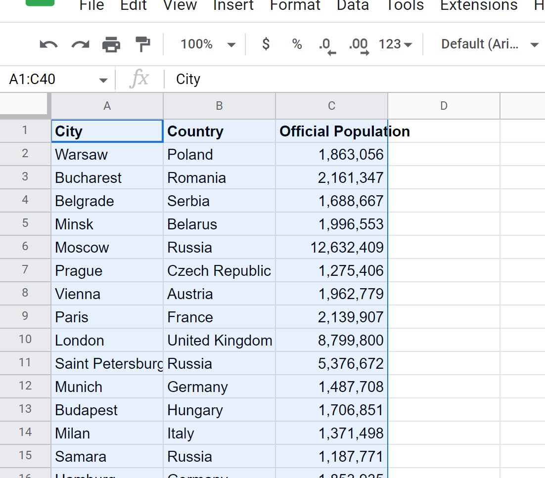
To select the data range, simply click and drag your mouse over the cells that contain the data you want to sort. You can select a single column, multiple columns, or even a range of cells that includes both columns and rows.
If your data is organized in a table format with headers, be sure to include the header row in your selection. This ensures that the header row remains intact as the data is sorted, providing clear labels for each column.
Once you have selected the data range, the cells you have chosen will be highlighted, making it easy for you to visually confirm that the correct data range has been selected. If you need to adjust your selection, simply click and drag again to include or exclude additional cells.
It is worth mentioning that Google Sheets also provides the option to sort multiple columns simultaneously. This can be useful when you have related data in different columns that you want to sort together. By selecting multiple columns, you can ensure that the integrity of your data is maintained during the sorting process.
Now that you have selected the data range you want to sort, let’s move on to the next step: accessing the “Data” menu.
Step 3: Click on the “Data” Menu
After selecting the data range you want to sort, the next step is to access the “Data” menu in Google Sheets. This menu contains various options for manipulating and organizing your data, including the ability to sort it alphabetically.
To access the “Data” menu, look at the toolbar at the top of the Google Sheets interface. Located between the “Format” and “Tools” menus, you will find the “Data” menu. Click on it to open a dropdown menu that displays a list of data-related options.
Once you have opened the “Data” menu, you will see a range of choices, including sorting options. In addition to sorting, this menu also provides options for filtering, grouping, and more. For our purposes, we will focus on the sorting functionality.
When you click on the “Data” menu, a list of options will appear. Scroll down the list until you find the “Sort range” option. This is the option we will be selecting to sort our data in alphabetical order.
By clicking on the “Sort range” option, you are indicating to Google Sheets that you want to rearrange your selected data based on a specific column. This will prompt a dialog box to appear, allowing you to further customize your sorting preferences.
Now that you know how to access the “Data” menu in Google Sheets, let’s move on to the next step: choosing the “Sort range” option.
Step 4: Choose “Sort Range”
After accessing the “Data” menu in Google Sheets, the next step is to choose the “Sort range” option. This option allows you to specify the sorting criteria for your selected data range, such as the column to sort by and the order of the sorting.
When you select the “Sort range” option from the “Data” menu, a dialog box will appear. This dialog box contains several options and settings that you can customize to suit your sorting needs.
In the dialog box, you will see a drop-down menu labeled “Sort by.” This menu displays a list of columns from your selected data range. Choose the column that you want to use as the basis for sorting your data. For example, if you want to sort a list of names alphabetically, select the column that contains the names.
Next, you will see a checkbox labeled “Data has header row.” If your data range includes a header row, make sure to check this box to indicate that the first row should not be included in the sorting process.
After selecting the column and specifying whether your data has a header row, you can choose the order in which you want the data to be sorted. Google Sheets provides two options: “A to Z” and “Z to A.” Select the option that best fits your needs.
Additionally, if you want to add a secondary sorting criterion, you have the option to choose another column in the “Then by” dropdown menu. This can be useful when you want to further refine the sorting order based on another column.
Once you have customized the sorting options in the dialog box, click the “Sort” button to apply the sorting to your selected data range. Google Sheets will rearrange your data based on the specified criteria, effectively sorting it in alphabetical order.
Now that you know how to choose the “Sort range” option in Google Sheets, let’s move on to the next step: selecting the column to sort by.
Step 5: Select the Column to Sort by
After choosing the “Sort range” option and customizing the sorting criteria in the dialog box, the next step is to select the specific column that you want to use as the basis for sorting your data. This column will determine the order in which your data is arranged.
In the dialog box that appears after selecting “Sort range,” you will see a drop-down menu labeled “Sort by.” This menu displays the columns from your selected data range. Choose the column that you want to use as the primary sorting criterion.
For example, if you have a spreadsheet with a list of names in one column and ages in another, and you want to sort the names alphabetically, select the column that contains the names as the sorting column.
It’s important to note that the column you select should contain data that is sortable in a meaningful way. For instance, if you have a column that contains numerical values, sorting by that column will arrange the data in numerical order.
Once you have selected the column to sort by, you can further refine the sorting order by choosing whether you want the data to be sorted in ascending order (A to Z) or descending order (Z to A). This option is available in the same dialog box.
Additionally, if you want to add a secondary sorting criterion, you can select another column in the “Then by” drop-down menu. This option allows you to specify a secondary column to sort by, which can be useful for sorting your data in a more granular way.
After selecting the column(s) and specifying the sorting order, click the “Sort” button in the dialog box to apply the sorting to your data. Google Sheets will rearrange your data based on the chosen column(s), effectively sorting it in the desired order.
Now that you know how to select the column to sort by, let’s move on to the next step: choosing the A to Z or Z to A order.
Step 6: Choose the A to Z or Z to A Order
After selecting the column to sort by in Google Sheets, the next step is to choose the order in which you want your data to be sorted. You have two options: A to Z or Z to A. Depending on your preference, you can choose the appropriate order to suit your needs.
In the dialog box that appears after selecting the column to sort by, you will see the option to choose the sorting order. By default, the “A to Z” option is selected, indicating that the data will be sorted in alphabetical order from A to Z.
If you want to reverse the sorting order and arrange the data from Z to A, simply select the “Z to A” option instead. This is particularly useful when you want to view your data in descending order or sort it in reverse alphabetical order.
It’s important to note that the sorting order you choose will apply to the selected column or columns. If you have selected multiple columns to sort by, all columns will be sorted in the same order.
Once you have chosen the desired sorting order, you can proceed to the next step: applying the sort to your data. This will rearrange your selected data range based on the column(s) and the chosen order, effectively sorting it in the desired sequence.
Sorting your data alphabetically can help you organize and analyze information more efficiently. By placing the data in a logical order, you can easily find specific entries, compare values, and identify patterns or trends in your data.
Now that you know how to choose the A to Z or Z to A order, let’s move on to the next step: applying the sort to your data.
Step 7: Apply the Sort
After selecting the column to sort by and choosing the desired sorting order in Google Sheets, the next step is to apply the sort to your selected data range. This will rearrange your data based on the specified criteria, effectively sorting it in the desired sequence.
To apply the sort, simply click the “Sort” button in the dialog box where you selected the column and sorting order. Google Sheets will then process the request and rearrange your data accordingly.
As soon as you click the “Sort” button, you will notice that your selected data range is automatically sorted based on the column and sorting order you specified. The rows will be reordered, with the data now displayed in the chosen sequence.
Google Sheets performs the sorting operation quickly and efficiently, regardless of the size of your data range. This allows you to sort even large datasets in a matter of seconds, enhancing your data analysis workflow and improving efficiency.
It’s important to note that applying the sort is a reversible action. If you decide later on that you want to return your data to its original order, you can simply undo or revert the sort operation. Google Sheets allows you to easily undo any changes made, ensuring that your data remains intact and unaltered.
Remember to review your sorted data to verify that it has been arranged correctly according to your chosen criteria. Take a moment to ensure that the sorting order, columns, and data range are accurate, especially if you have selected multiple columns or added secondary sorting criteria.
Once you have applied the sort and confirmed that your data is correctly organized, you can proceed to the next step: refreshing the sort if needed. This will allow you to update and maintain the sorted order as you make changes or add new data to your spreadsheet.
Step 8: Refresh the Sort
After applying the sort to your data in Google Sheets, it’s important to refresh the sort if you make any changes or additions to your spreadsheet. This ensures that your sorted data remains up to date and accurately reflects any modifications you make.
When you refresh the sort, Google Sheets will reapply the sorting criteria to your data range, taking into account any changes or new entries. This helps you maintain the integrity and accuracy of your sorted data, especially when working with dynamic or constantly evolving datasets.
To refresh the sort in Google Sheets, simply follow these steps:
- Make any necessary changes or additions to your data. This could involve modifying existing entries, adding new rows or columns, or inputting fresh data.
- Click anywhere within your sorted data range to select it.
- In the toolbar at the top of the Google Sheets interface, click on the “Data” menu.
- From the dropdown menu, select the “Sort range” option.
- In the dialog box that appears, review the sorting options and make sure they match your desired criteria.
- Click the “Sort” button to reapply the sort to your updated data range.
By following these steps, you will refresh the sort in Google Sheets and ensure that your sorted data accurately reflects any changes or additions you have made.
Refreshing the sort is especially useful when you are working with real-time data or frequently updating your spreadsheet. It allows you to maintain an organized and up-to-date view of your data, making it easier to analyze and interpret.
Now that you know how to refresh the sort in Google Sheets, you can confidently manage and update your sorted data as needed.
Conclusion
Sorting data alphabetically in Google Sheets is a straightforward process that can greatly enhance your data management and analysis capabilities. By following the step-by-step instructions outlined in this article, you can easily arrange your data in a logical order, making it easier to find, compare, and analyze information.
We started by opening Google Sheets and selecting the data range that we wanted to sort. Then, we accessed the “Data” menu and chose the “Sort range” option to initiate the sorting process. From there, we selected the column to sort by, whether it was names, numbers, or any other relevant information. We also had the option to customize the sort order, choosing between A to Z or Z to A.
After customizing the sorting criteria, we applied the sort and saw our data rearranged accordingly. It’s important to remember that we can always refresh the sort if changes or additions are made to the spreadsheet. This ensures that our sorted data remains accurate and up to date.
Sorting data alphabetically in Google Sheets offers numerous benefits, including improved organization, easier data analysis, and efficient retrieval of information. Whether you’re working with lists, customer data, or any other type of data, sorting it alphabetically can provide valuable insights, save time, and enhance productivity.
By mastering the art of sorting data in Google Sheets, you can unlock the full potential of the application and make the most of your data. So, go ahead and apply the techniques learned in this article to make your Google Sheets more organized and user-friendly.
Overall, sorting data alphabetically in Google Sheets is an essential skill for anyone working with spreadsheets. It allows you to easily navigate and manipulate large sets of data, making it more comprehensible and usable. So why wait? Start sorting your data in Google Sheets and experience the benefits for yourself!