Introduction
Dropdown menus are a useful and interactive feature that can be incorporated into Google Sheets to enhance data entry and organization. Whether you are creating a form, survey, or managing a spreadsheet, dropdown menus can provide a streamlined user experience by allowing users to choose from a set list of options.
In this article, we will guide you through the steps to create a dropdown menu in Google Sheets. Whether you are a beginner or an experienced user, this step-by-step tutorial will help you add this valuable feature to your spreadsheets and improve data entry efficiency.
By utilizing dropdown menus in Google Sheets, you can ensure data consistency, reduce human error, and make data entry a breeze. Instead of manually typing in specific values, users can easily select the desired option from a predetermined list, eliminating the risk of typos or incorrect entries. Dropdown menus can be particularly useful in situations where there are predefined categories or options that users need to choose from.
Whether you want to create a dropdown menu for selecting products, assigning priority levels, or choosing region locations, this guide will walk you through the process step by step. So let’s dive in and learn how to create a dropdown menu in Google Sheets!
Step 1: Open Google Sheets
Before you can create a dropdown menu in Google Sheets, you need to open the application. To begin, open your web browser and navigate to the Google Sheets website. If you have a Google account, sign in; otherwise, create a new account to access Sheets.
Once you are signed in, click on the Google Apps menu (usually represented by nine small squares in the top right corner of the window) and select “Sheets” from the available apps. Alternatively, you can directly type “sheets.google.com” into your browser’s address bar to go directly to Google Sheets.
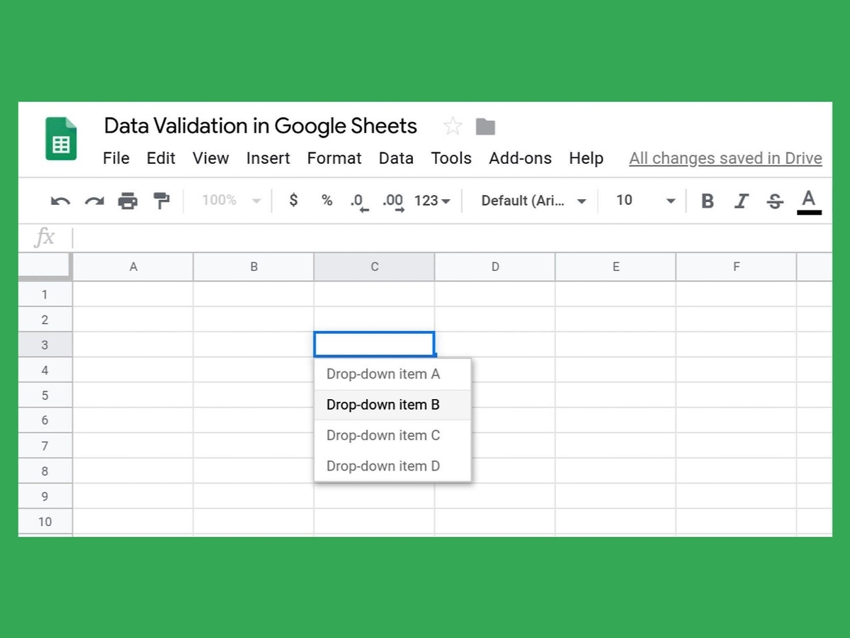
Google Sheets will now open in a new tab or window. You will be presented with a blank sheet, ready for you to begin adding data and creating your dropdown menu.
It’s worth noting that Google Sheets offers both a web-based version and a desktop application. The steps outlined in this tutorial apply to both. Whether you are using the web-based version in your browser or the desktop application, you can follow along and create dropdown menus seamlessly.
Now that you have opened Google Sheets, you are ready to move on to the next step and start creating your dropdown menu. Let’s dive into creating your spreadsheet and adding the dropdown functionality!
Step 2: Create a new or open an existing spreadsheet
Once you have opened Google Sheets, you have the option to create a new spreadsheet or open an existing one. If you already have a specific spreadsheet that you want to add a dropdown menu to, open it by navigating through your Google Drive or using the “Open” option in Google Sheets.
If you don’t have an existing spreadsheet or want to create a new one, you can do so by clicking on the “Blank” option when you first open Google Sheets. This will create a new, empty spreadsheet for you to work with.
Once you have either opened an existing spreadsheet or created a new one, you will be presented with a grid-like interface where you can enter and manipulate data. Each cell in the spreadsheet is identified by a unique combination of columns and rows, such as A1, B2, or C7. You can navigate through the cells by clicking on them or using the arrow keys on your keyboard.
The spreadsheet provides a flexible and customizable workspace where you can enter and organize your data. You can add columns and rows, format the cells, apply formulas, and much more. It’s important to have a clear understanding of your data structure and the purpose of your spreadsheet before proceeding to create a dropdown menu.
Now that you have either opened an existing spreadsheet or created a new one, you are ready to move on to the next step and select the cell or cells where you want to create the dropdown menu. Let’s continue with the tutorial and add dropdown functionality to your spreadsheet!
Step 3: Select the cell or cells where you want to create the dropdown
Before you can create a dropdown menu in Google Sheets, you need to select the cell or range of cells where you want the dropdown to be displayed. This is where users will be able to choose from the predefined options.
To select a single cell, simply click on it. The selected cell will be outlined or highlighted to indicate that it is currently active.
If you want to select a range of cells, click and hold on one cell, then drag your cursor to select the adjacent cells. The selected cells will be highlighted together as a range.
Keep in mind that the dropdown menu will be displayed in the selected cell or cells, so it’s important to choose the appropriate location in your spreadsheet.
Depending on your specific needs, you can create multiple dropdown menus in different cells or have one dropdown menu that spans across a range of cells. The choice is entirely up to you and the purpose of your spreadsheet.
By selecting the cell or cells where you want to create the dropdown, you are now ready to move on to the next step and access the data validation feature in Google Sheets. Let’s continue with the tutorial and learn how to create your dropdown menu!
Step 4: Go to the Data tab
Once you have selected the cell or range of cells where you want to create the dropdown menu, it’s time to access the data validation feature in Google Sheets. Data validation allows you to define rules and restrictions for the selected cell or cells, including the option to create a dropdown menu.
To access the data validation feature, navigate to the “Data” tab at the top of the Google Sheets interface. Click on the “Data” tab to reveal a dropdown menu with various options.
The “Data” tab offers a range of features and tools to manipulate and format your data. In this tutorial, we will specifically focus on the data validation feature to create the dropdown menu.
By clicking on the “Data” tab, you will be able to access the necessary tools to define the criteria and options for your dropdown menu. This includes specifying the source of the dropdown options and customizing the behavior of the dropdown.
Now that you have navigated to the “Data” tab, you are ready to move on to the next step and click on the data validation option. Let’s continue with the tutorial and learn how to create your dropdown menu in Google Sheets!
Step 5: Click on Data Validation
After accessing the “Data” tab in Google Sheets, the next step is to click on the “Data Validation” option. This will open a dialog box where you can configure the settings for the dropdown menu.
When you click on “Data Validation,” a window will appear with various tabs and options. This is where you will define the criteria and behavior of the dropdown menu.
Within the “Data Validation” window, you will see multiple tabs, including “Criteria,” “Input Message,” and “Error Message.” These tabs allow you to set specific criteria for the dropdown menu, customize the input message that appears when a user selects the cell, and specify an error message for invalid entries.
In the “Criteria” tab, you have several options to choose from. To create a dropdown menu, select the option “List from a range.” This will enable you to specify the range of cells that contain the dropdown options.
By clicking on “Data Validation” and accessing the various tabs, you have now opened the door to customizing and fine-tuning your dropdown menu. The “Data Validation” window provides a user-friendly interface where you can define the behavior and appearance of your dropdown menu.
Now that you have clicked on “Data Validation” and opened the settings window, you are ready to proceed to the next step and specify the range of cells that contain the dropdown options. Let’s continue with the tutorial and learn how to create your dropdown menu in Google Sheets!
Step 6: Choose “List from a range” for the “Criteria” option
After opening the “Data Validation” window, the next step is to choose the “List from a range” option for the “Criteria” setting. This option allows you to specify the range of cells that contain the dropdown options you want to display.
When you select “List from a range,” a new input field will appear where you can enter the range of cells. This range should contain the options that will be displayed in the dropdown menu.
To specify the range, you can manually enter the cell references in the input field. For example, if your dropdown options are located in cells A1 to A4, you would enter “A1:A4” in the input field. Alternatively, you can click on the small icon next to the input field to select the range visually by highlighting the cells on your spreadsheet.
It’s important to note that the range you specify should only include the cells with the dropdown options and not any additional data. Make sure to double-check the range to ensure that you have selected the correct cells.
By choosing “List from a range” for the “Criteria” option, you are telling Google Sheets that you want to display a dropdown menu with the options from the specified range. This gives you full control over the content of the dropdown menu and allows users to choose from the predefined options you have provided.
Now that you have chosen “List from a range” for the “Criteria” option, you are ready to move on to the next step and enter the range of cells that contain the dropdown options. Let’s continue with the tutorial and create your dropdown menu in Google Sheets!
Step 7: Enter the range of cells that contain the dropdown options
Once you have selected “List from a range” for the “Criteria” option in the “Data Validation” window, the next step is to enter the range of cells that contain the dropdown options you want to display.
To specify the range of cells, click on the input field next to the “List from a range” option. This will allow you to manually enter the cell references or visually select the range using your mouse.
If you prefer to manually enter the range, you can simply type the cell references in the input field. For example, if your dropdown options are located in cells A1 to A4, you would enter “A1:A4” in the input field.
Alternatively, you can visually select the range by clicking on the small icon next to the input field. This will activate a selection tool that allows you to click and drag your mouse to highlight the cells containing the dropdown options.
Make sure to double-check the entered range to ensure it is accurate and includes only the cells you want to display in the dropdown menu. If there are any extra cells included in the range, you can manually adjust the range before proceeding.
By entering the range of cells that contain the dropdown options, you are specifying the content of the dropdown menu. Users will be able to select from the options within this range when they interact with the dropdown menu.
Now that you have entered the range of cells, you are ready to move on to the next step and choose whether to show a dropdown arrow or not. Let’s continue with the tutorial and create your dropdown menu in Google Sheets!
Step 8: Select whether to show a dropdown arrow or not
After entering the range of cells that contain the dropdown options, the next step is to decide whether to show a dropdown arrow in the selected cell or cells. The dropdown arrow provides a visual indication that the cell has a dropdown menu attached to it.
In the “Data Validation” window, you will find an option called “Show dropdown list in cell.” By default, this option is enabled, meaning that a dropdown arrow will be displayed in the selected cell or cells.
If you prefer not to show the dropdown arrow, you can simply uncheck the box next to the “Show dropdown list in cell” option. This will hide the visual indicator in the cell, giving it a cleaner and more streamlined appearance.
Keep in mind that even if you choose not to show the dropdown arrow, the dropdown functionality will still be active. Users can still click on the cell to reveal the dropdown menu and select an option from the list.
Deciding whether or not to show the dropdown arrow is a matter of personal preference and depends on the visual aesthetics and usability of your spreadsheet. Consider the overall design and functionality of your sheet before making a decision.
By selecting whether to show a dropdown arrow or not, you have now customized the appearance of your dropdown menu. You are almost done with creating your dropdown menu in Google Sheets!
Now that you have made a decision about showing the dropdown arrow or not, you are ready to move on to the next step and choose whether to display a warning message or reject invalid entries. Let’s continue with the tutorial and complete the creation of your dropdown menu!
Step 9: Choose whether to display a warning message or reject invalid entries
Once you have selected the options for the dropdown arrow, the next step is to decide whether to display a warning message or reject invalid entries. This feature helps ensure that users enter only valid data that aligns with the predefined dropdown options.
In the “Data Validation” window, you will find two tabs: “Input Message” and “Error Message.” These tabs allow you to customize the messages that appear when a user interacts with the dropdown menu.
The “Input Message” tab provides an opportunity to display a custom message when a user selects the cell with the dropdown menu. This message can provide guidance or instructions for using the dropdown menu.
The “Error Message” tab is crucial for maintaining data integrity. Here, you can choose whether to display an error message when a user enters data that is not in the predefined dropdown options. You can customize the error message to inform the user about the invalid entry.
If you want to allow users to input values that are not in the dropdown options, you have the option to show a warning message instead of rejecting the entry. The warning message can inform the user about the potential discrepancy between the entered value and the predefined options.
By choosing whether to display a warning message or reject invalid entries, you can ensure data accuracy and guide users in entering the appropriate information within the defined parameters of the dropdown menu.
Now that you have made a decision about displaying a warning message or rejecting invalid entries, you are ready to proceed to the next step and save your settings. Let’s move forward and finalize the creation of your dropdown menu in Google Sheets!
Step 10: Click on Save
After customizing the settings for your dropdown menu in the “Data Validation” window, the final step is to click on the “Save” button. This will apply the changes you have made and create the dropdown menu in the selected cell or cells.
By clicking on “Save,” Google Sheets will validate your settings and ensure that they are properly configured. If there are any errors or conflicts, a notification will be displayed, allowing you to review and correct them before saving.
Once you have clicked on “Save,” the specified cell or cells will now have a dropdown menu attached to them. Users can click on the cell to reveal the dropdown menu and select an option from the list.
It’s important to note that by saving the changes, the dropdown menu becomes an integral part of your spreadsheet. Any changes to the dropdown options or settings will require modifying the data validation settings again.
If you need to make any adjustments to the dropdown menu, such as adding or removing options, modifying the range, or changing the display settings, you can simply repeat the steps outlined in this tutorial.
Now that you have clicked on “Save” and created your dropdown menu, you are ready to start using and benefiting from this interactive feature in your Google Sheets spreadsheet.
Congratulations! You have successfully completed all the steps to create a dropdown menu in Google Sheets. Enjoy the improved data entry and organization that this feature provides!
Conclusion
Creating a dropdown menu in Google Sheets is a straightforward process that can greatly enhance the usability and efficiency of your spreadsheets. By allowing users to select from a predefined list of options, dropdown menus promote data consistency, reduce errors, and improve the overall user experience.
In this tutorial, we covered the step-by-step process of creating a dropdown menu in Google Sheets. We started by opening Google Sheets and selecting the desired cell or cells where the dropdown menu should be displayed. Then, we accessed the “Data” tab and clicked on “Data Validation” to configure the settings for the dropdown menu.
We learned how to choose “List from a range” for the “Criteria” option and enter the range of cells that contain the dropdown options. We also explored the option of showing or hiding the dropdown arrow and deciding whether to display a warning message or reject invalid entries.
Finally, after customizing all the settings, we clicked on “Save” to create the dropdown menu in our spreadsheet. With the dropdown menu in place, users can effortlessly select options from the list, ensuring accurate and consistent data entry.
Remember, dropdown menus can be easily modified and customized to fit your specific needs. You can update the range of cells, add or remove options, or adjust the display settings as necessary.
By incorporating dropdown menus in your Google Sheets spreadsheets, you can streamline data entry, enhance organization, and optimize the overall efficiency of your work. Take advantage of this powerful feature to make your spreadsheets more user-friendly and productive.
Now that you have mastered the art of creating dropdown menus in Google Sheets, go ahead and explore the endless possibilities to improve your data management and analysis!