Introduction
Adding borders to your Google Sheets can help enhance the visual appeal and organization of your data. Whether you want to highlight specific cells, create boundaries between sections, or make your spreadsheet easier to read, borders can be a valuable tool.
In this article, you will learn several methods for adding borders in Google Sheets. Whether you prefer using the toolbar, the Format menu, keyboard shortcuts, or conditional formatting, we’ve got you covered. So, let’s dive in and explore the various ways to add borders to your Google Sheets.
Whether you’re a student, a professional, or just an everyday user of Google Sheets, understanding how to add borders can greatly improve the presentation and functionality of your spreadsheets. Borders can help you quickly identify important information, organize data, and enhance the overall readability of your sheet.
Now that you know the importance of adding borders in Google Sheets, let’s explore the different methods available to make your data standout.
Method 1: Using the toolbar
One of the easiest ways to add borders in Google Sheets is by using the toolbar. The toolbar is conveniently located at the top of the screen and offers a variety of formatting options, including the ability to add borders to your cells.
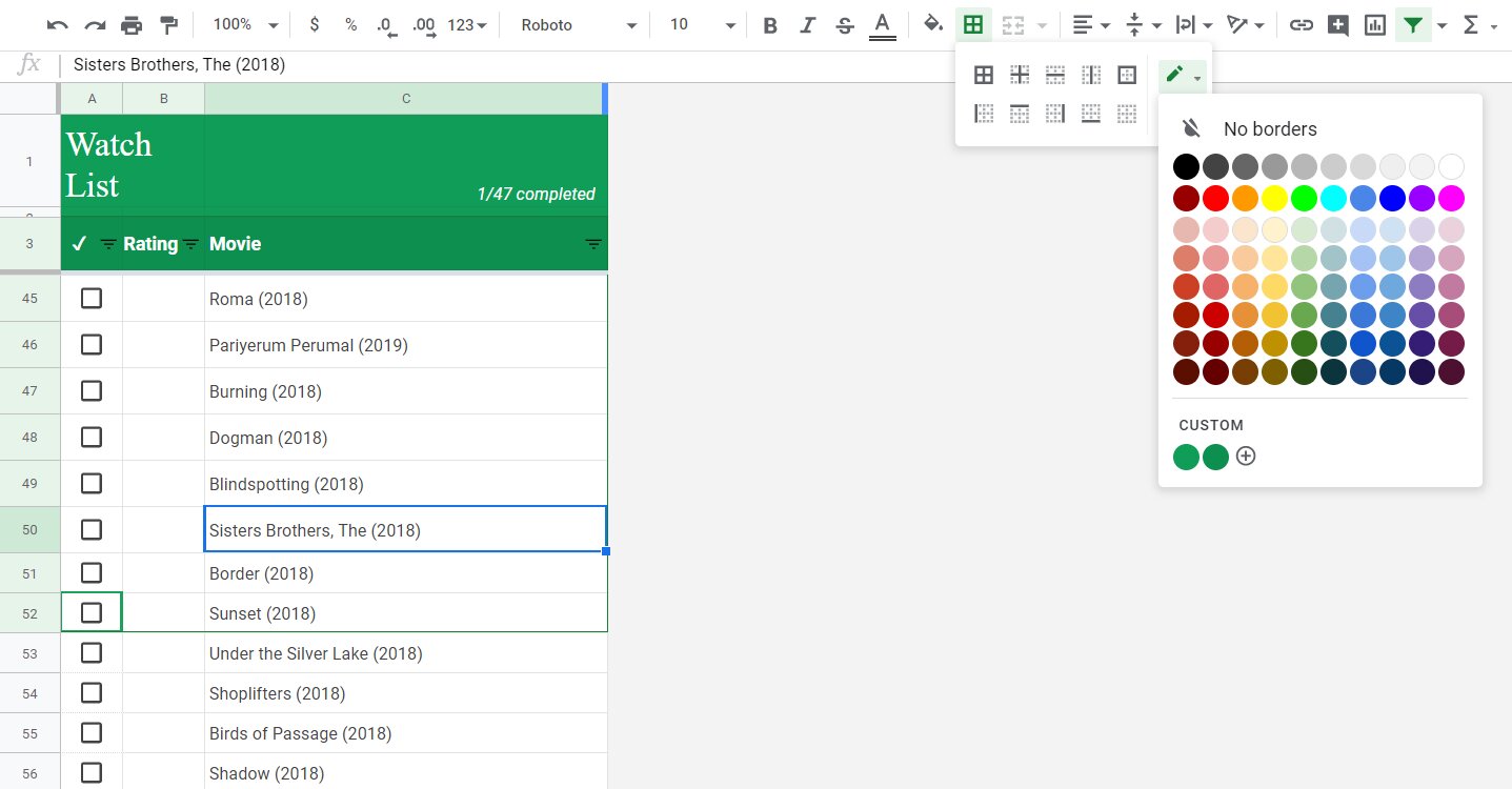
To begin, open your Google Sheets document and select the cells to which you want to add borders. You can do this by clicking and dragging your cursor over the desired cells. Once the cells are selected, navigate to the toolbar and locate the “Borders” icon. It typically looks like a square divided into four smaller squares.
Click on the “Borders” icon to access the border formatting options. A dropdown menu will appear, displaying various border styles, such as solid lines, dashed lines, and dotted lines. You can also choose the thickness of the borders, ranging from thin to thick.
To add a border to your selected cells, simply click on the desired border style in the dropdown menu. The border will be applied immediately, allowing you to see the visual representation of the border before finalizing your selection. Repeat this process if you want to add different border styles or thicknesses to different sides of the cells.
If you want to remove borders from your cells, you can select the cells again, click on the “Borders” icon, and choose “Clear borders” from the dropdown menu. This will remove all borders from the selected cells.
Using the toolbar to add borders in Google Sheets is quick and straightforward. It provides you with an array of border styles and thicknesses to choose from, allowing you to customize the appearance of your cells to suit your needs.
Now that you’ve learned how to add borders using the toolbar, let’s explore another method for adding borders in Google Sheets.
Method 2: Using the Format menu
Another way to add borders in Google Sheets is by utilizing the options provided in the Format menu. This method offers additional customization features that can help you create more sophisticated border styles.
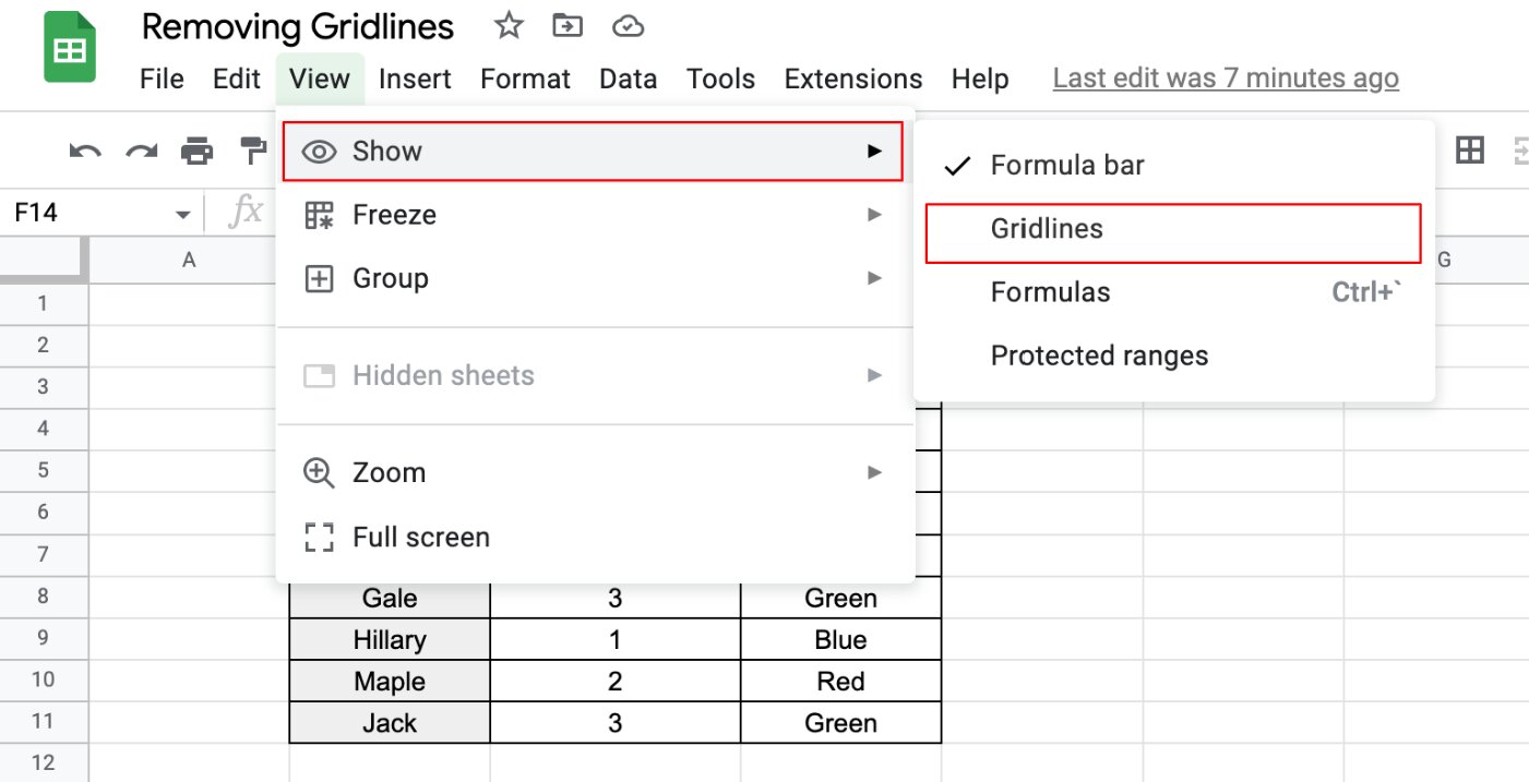
To get started, open your Google Sheets document and select the cells to which you want to apply borders. Once the cells are selected, navigate to the top menu and click on “Format.” A dropdown menu will appear, and you’ll need to hover over the “Borders” option.
When you hover over the “Borders” option, a secondary menu will appear, presenting you with various border styles and customization options. You can choose from options like “Top border,” “Bottom border,” “Full border,” and more.
Click on the specific border option you want to apply to your selected cells. A pop-up window will appear, allowing you to further customize the border style. You can choose the line style, color, and thickness by selecting the appropriate options in the pop-up window.
If you want to apply the same border style to multiple sides of the cells, you can use the “Full border” option from the primary “Borders” menu. This will apply borders to all four sides of the selected cells, creating a complete border around them.
To remove borders, select the cells again, navigate to the “Borders” option, and choose the “None” option from the secondary menu. This will remove all borders from the selected cells.
Using the Format menu provides you with more precise control over the borders in Google Sheets. It allows you to customize each side of the cells individually and apply various border styles to create visually appealing spreadsheets.
Now that you’ve discovered how to add borders using the Format menu, let’s explore another method for adding borders in Google Sheets.
Method 3: Using keyboard shortcuts
If you’re a fan of using keyboard shortcuts to navigate and format your spreadsheets more efficiently, Google Sheets offers several shortcuts specifically designed for adding borders.
To start, open your Google Sheets document and select the cells to which you want to add borders. You can do this by clicking and dragging your cursor over the desired cells. Once the cells are selected, use the following keyboard shortcuts based on your operating system:
- For Windows and Linux: Press Ctrl + Alt + Shift + Borders simultaneously.
- For Mac: Press ⌘ + Option + Shift + Borders simultaneously.
After pressing the corresponding keyboard shortcut, a sidebar will appear on the right side of the screen, displaying various border options. You can choose the desired border style, thickness, and color from the available options in the sidebar.
Using keyboard shortcuts not only saves time by eliminating the need to navigate through menus, but it also provides a quick and efficient way to add borders to your cells. These shortcuts are especially handy for users who prefer to keep their hands on the keyboard while working.
To remove borders using keyboard shortcuts, select the cells with borders and use the following keyboard shortcuts:
- For Windows and Linux: Press Ctrl + Alt + Shift + & simultaneously.
- For Mac: Press ⌘ + Option + Shift + & simultaneously.
This will remove all the borders from the selected cells, allowing you to start fresh or apply new border styles.
Now that you know how to add and remove borders using keyboard shortcuts, let’s move on to another method for adding borders in Google Sheets.
Method 4: Using conditional formatting
Conditional formatting is a powerful feature in Google Sheets that allows you to automatically apply formatting, including borders, based on specific conditions or criteria. This method is particularly useful when you want to add borders to cells dynamically based on certain rules.
To utilize conditional formatting to add borders, follow these steps:
- Select the cells to which you want to apply the conditional formatting.
- From the top menu, click on “Format” and select “Conditional formatting” from the dropdown menu.
- In the “Conditional format rules” sidebar that appears on the right, choose the condition based on which you want to add borders. For example, “Greater than,” “Less than,” “Text contains,” etc.
- Specify the rule criteria and select the border style, thickness, and color you desire.
- Click “Done” to apply the conditional formatting with borders to the selected cells.
Conditional formatting allows you to add borders dynamically, making it easy to highlight specific data points based on your desired criteria. You can create multiple conditional formatting rules with different border styles to provide clearer visual cues in your spreadsheet.
To remove conditional formatting with borders, select the cells with conditional formatting, navigate back to the “Conditional formatting” option under the “Format” menu, and choose the “Clear rules” option. This will remove all the conditional formatting rules, including the borders, from the selected cells.
By utilizing conditional formatting, you can add borders to your cells automatically based on specific conditions, allowing for a more dynamic and visually appealing spreadsheet.
Now that you’ve learned how to apply borders using conditional formatting, let’s wrap up and summarize what you’ve learned.
Conclusion
Adding borders in Google Sheets is a simple yet effective way to enhance the visual appeal and organization of your data. In this article, we explored four different methods for adding borders: using the toolbar, utilizing the Format menu, using keyboard shortcuts, and applying conditional formatting.
The toolbar offers a quick and convenient way to add borders with various styles and thicknesses. The Format menu provides more customization options, allowing you to create sophisticated border styles. Keyboard shortcuts are perfect for users who prefer a hands-on approach and want to navigate and format their spreadsheets efficiently. Conditional formatting lets you dynamically apply borders based on specific conditions or criteria.
By adding borders to your Google Sheets, you can quickly identify important information, create boundaries between sections, and improve readability. Borders help highlight data and make your spreadsheet visually appealing and organized.
Remember, there is no one-size-fits-all method for adding borders in Google Sheets. Choose the method that suits your preferences and workflow the best. Experiment with different border styles, colors, and thicknesses to find the perfect combination for your data.
Now that you’ve mastered the art of adding borders in Google Sheets, you can take your spreadsheets to the next level. With the newfound knowledge and skills, your data will be more visually engaging and easier to interpret.
So, go ahead and start applying borders to your Google Sheets. Let your creativity shine and make your data stand out!