How To Remove Grid Lines In Google Sheets

Introduction

Welcome to this tutorial on how to remove grid lines in Google Sheets. Google Sheets is a powerful spreadsheet software that allows you to organize data, perform calculations, and create visually appealing presentations. Grid lines are the horizontal and vertical lines that separate cells in a sheet, making it easier to read and navigate your data.

While grid lines can be useful for maintaining structure and alignment, sometimes you may want to remove them to enhance the visual clarity of your spreadsheet. Whether you are creating a professional report, a sleek design, or simply prefer a cleaner look, removing grid lines can help you achieve the desired aesthetic.

In this guide, we will explore several methods to remove grid lines in Google Sheets. We will cover various approaches, including using the View menu, keyboard shortcuts, the Format menu, the Formatting toolbar, the Gridlines option, and even Conditional Formatting. By following these methods, you will have the flexibility to customize your sheet and improve its appearance to meet your specific needs.

Why Remove Grid Lines

Grid lines can be a helpful visual aid when working with spreadsheets, providing a clear separation between cells and rows. However, there are several reasons why you might want to remove grid lines in Google Sheets:

1. Aesthetics: Removing grid lines can give your spreadsheet a cleaner, more professional appearance. This can be particularly important when presenting data to clients, colleagues, or stakeholders. By removing distracting grid lines, your audience can focus on the content and analysis within your sheet.

2. Design Flexibility: Grid lines can sometimes limit your design options, especially when you want to create visually appealing presentations or reports. By removing grid lines, you can have more control over formatting, such as merging cells to create customized layouts or inserting images without the constraints of the grid lines.

3. Enhancing Readability: In certain cases, grid lines can make it harder to read data, especially when working with large spreadsheets. Removing grid lines can improve readability, particularly when you have a dense collection of data or complex formulas in your sheet. This can help you quickly identify patterns, trends, and outliers.

4. Focus on Data Insights: Grid lines can sometimes distract from the actual data in your sheet. By removing them, you can emphasize the important information and insights you want to convey. Whether you are analyzing financial data, conducting statistical analysis, or creating a dashboard, removing grid lines can help your audience focus on the meaningful aspects of your spreadsheet.

5. Customization: Removing grid lines allows you to customize the appearance and layout of your sheet. You can experiment with different color schemes, fonts, and formatting options to make your spreadsheet more visually appealing and align with your personal or brand preferences.

In summary, while grid lines serve a purpose in organizing and reading data, removing them can offer a range of benefits, from improving aesthetics and design flexibility to enhancing readability and focusing on data insights. Google Sheets provides multiple methods to remove grid lines, ensuring you have the freedom to create visually appealing and informative spreadsheets.

Method 1: Using the View Menu

Removing grid lines in Google Sheets is a simple process, and one way to accomplish this is by using the View menu. Follow these steps:

1. Open your Google Sheets document.
2. Click on the “View” tab in the top menu.
3. In the dropdown menu, uncheck the “Gridlines” option.

By unchecking the “Gridlines” option, the grid lines in your spreadsheet will disappear, giving it a cleaner and more streamlined appearance.

This method is ideal if you want to quickly toggle the visibility of grid lines on and off. It is especially useful when you need to remove grid lines temporarily for presenting or sharing your spreadsheet, as you can easily enable them again using the same steps.

Note that by using this method, you are only hiding the grid lines visually. The cells will still retain their original formatting and align correctly, but the grid lines will no longer be visible.

Using the View menu to remove grid lines is a straightforward and efficient method to enhance the visual appeal and readability of your Google Sheets document. However, there are other methods available as well, which we will explore in the following sections.

Method 2: Using Keyboard Shortcuts

If you prefer to use keyboard shortcuts for quick and efficient navigation in Google Sheets, you’ll be pleased to know that there is a shortcut to remove grid lines as well. Here’s how:

1. Open your Google Sheets document.
2. Press the Ctrl + Alt + Shift + 7 keys simultaneously on Windows or Cmd + Option + Shift + 7 on Mac.

By using this keyboard shortcut, you can swiftly remove grid lines from your spreadsheet without the need to navigate through any menus or options.

Similar to the previous method, removing grid lines using keyboard shortcuts visually hides the grid lines while retaining the formatting and alignment of the cells.

Keyboard shortcuts are a convenient way to perform actions quickly, particularly for those who prefer using the keyboard over the mouse. By utilizing this method, you can efficiently remove grid lines in Google Sheets, saving you time and effort in the process.

While the keyboard shortcut method works well for removing grid lines, there are more options available that we will explore in the upcoming sections.

Method 3: Using the Format Menu

Another way to remove grid lines in Google Sheets is by using the Format menu. Follow these steps:

1. Open your Google Sheets document.
2. Select the range of cells from which you want to remove the grid lines.
3. Click on the “Format” tab in the top menu.
4. In the dropdown menu, hover over “Borders and lines” and select “No borders”.

By choosing “No borders” from the “Borders and lines” section, you remove all the grid lines within the selected range of cells.

This method allows you to have more control over which areas of your spreadsheet have grid lines removed. You can select specific ranges or the entire sheet, depending on your preferences and requirements.

Using the Format menu to remove grid lines provides you with flexibility in customizing the appearance of your Google Sheets document. You can remove grid lines from specific areas while leaving them intact in other parts of the sheet, allowing for a more visually appealing and organized presentation of your data.

Now that you are familiar with using the Format menu to remove grid lines, let’s explore another method in the following section.

Method 4: Using the Formatting Toolbar

Removing grid lines in Google Sheets can also be achieved using the Formatting toolbar. Follow these steps:

1. Open your Google Sheets document.
2. Select the range of cells from which you want to remove the grid lines.
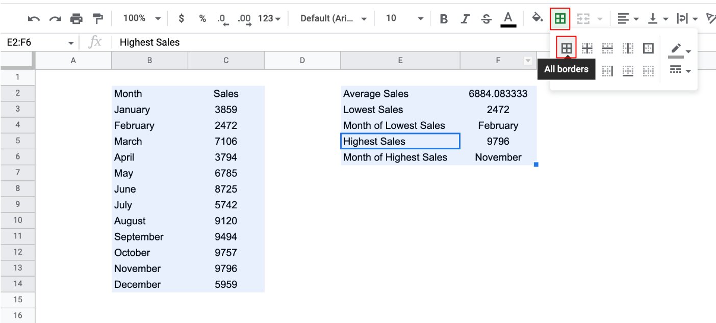
3. In the Formatting toolbar at the top, locate the “Borders” icon represented by a small square divided into four sections.
4. Click on the drop-down arrow next to the Borders icon.
5. In the drop-down menu, click on “No borders”.

By selecting “No borders” from the Borders drop-down menu, you will remove all the grid lines within the selected range of cells.

The Formatting toolbar provides a convenient and quick way to access formatting options, including removing grid lines. It allows you to remove grid lines in specific ranges and customize the appearance of your spreadsheet as desired.

This method is particularly useful when you want to remove grid lines from specific sections of your sheet or make quick formatting changes without navigating through menus. With just a few clicks, you can achieve a polished and professional look for your Google Sheets document.

Now that you have learned how to remove grid lines using the Formatting toolbar, let’s move on to exploring another method in the next section.

Method 5: Using the Gridlines Option

Google Sheets provides a dedicated option to control the visibility of grid lines. You can easily toggle the gridlines on or off using this feature. Here’s how:

1. Open your Google Sheets document.
2. Click on the “View” tab in the top menu.
3. In the dropdown menu, click on “Gridlines” to toggle the visibility.

By clicking on the “Gridlines” option, you can show or hide grid lines in your spreadsheet as needed.

This method offers a quick way to toggle the visibility of grid lines without affecting the formatting or content of your cells. It is especially useful when you want to temporarily hide the grid lines for a better view of your data, or when you need to enable them again for editing or sharing purposes.

Using the Gridlines option gives you the flexibility to showcase grid lines when desired or remove them to focus on the content and analysis of your Google Sheets document.

Now that you are familiar with using the Gridlines option to control the visibility of grid lines, let’s explore another method in the following section.

Method 6: Using Conditional Formatting

In Google Sheets, you can also remove grid lines using Conditional Formatting, which allows you to apply formatting rules to specific cells based on certain conditions. Here’s how you can remove grid lines using this method:

1. Open your Google Sheets document.
2. Select the range of cells from which you want to remove the grid lines.
3. Click on the “Format” tab in the top menu.
4. In the dropdown menu, select “Conditional formatting”.
5. In the Conditional Formatting sidebar, choose “Custom formula is” as the rule type.
6. In the custom formula field, enter the formula “=FALSE”.
7. Select the desired formatting style, such as “None” for border.
8. Click the “Done” button to apply the conditional formatting.

By applying the custom formula “=FALSE” as the conditional formatting rule, you are essentially removing the grid lines in the selected range.

This method is particularly useful if you want more control over when and where to remove the grid lines. You can specify specific conditions or criteria for the removal of grid lines, such as based on certain numerical values, text patterns, or other criteria that apply to your data.

Using Conditional Formatting to remove grid lines gives you the flexibility to tailor the appearance of your spreadsheet based on specific conditions, ensuring that your data is presented in a visually appealing and organized manner.

Now that you have learned how to remove grid lines using Conditional Formatting, let’s summarize the methods discussed in the next section.

Conclusion

Removing grid lines in Google Sheets can significantly enhance the visual appeal and readability of your spreadsheets. Throughout this tutorial, we explored different methods to remove grid lines, offering you various approaches to customize the appearance of your Google Sheets document.

We started by using the View menu and keyboard shortcuts to quickly toggle the grid lines on and off. These methods are ideal for temporary removal of grid lines or when you need a quick way to enable or disable them.

We then moved on to using the Format menu and the Formatting toolbar, which provide more control over the removal of grid lines in specific ranges of cells. These methods allow you to customize the appearance of your spreadsheet by selectively removing grid lines.

Using the Gridlines option in the View menu allows you to easily show or hide grid lines with a single click, providing flexibility when you need to temporarily remove grid lines from the entire document.

Lastly, we explored using Conditional Formatting to remove grid lines based on specific conditions. This approach offers a more advanced way to customize the appearance of your spreadsheet by removing grid lines based on certain criteria or rules.

By utilizing these methods, you have the flexibility to tailor your Google Sheets document to your needs and preferences, whether you want a clean and professional look, better readability, or more design flexibility.

Remember that even though grid lines are not visible, the cell formatting and data alignment remain unchanged, ensuring that your spreadsheet remains organized and functional.

Now that you are equipped with the knowledge to remove grid lines in Google Sheets, you can confidently create polished and visually appealing spreadsheets that showcase your data effectively.