How To Merge Two Columns In Google Sheets

Introduction

Welcome to this guide on how to merge two columns in Google Sheets. Google Sheets is a powerful tool for organizing and manipulating data, and sometimes you may need to combine multiple columns into one for better data analysis or presentation. Whether you are working on a spreadsheet for personal or professional use, merging columns can help streamline your data and make it easier to work with.

Merging columns in Google Sheets allows you to consolidate information from different columns into a single column, making it more convenient to view and analyze data. This process is particularly useful when dealing with spreadsheets that have data distributed across multiple columns, such as when you have first names in one column and last names in another. By merging these columns, you can create a single column containing the full names.

Throughout this step-by-step guide, we will walk you through the process of merging two columns in Google Sheets. You will learn how to select the columns you want to merge, how to perform the merge operation, and how to adjust the merged column to fit your needs. So let’s get started and learn how to merge columns in Google Sheets!

Step 1: Open Google Sheets

The first step in merging two columns in Google Sheets is to open the Google Sheets application. If you don’t already have a Google Sheets document that contains the columns you want to merge, you can create a new one by following these simple steps:

1. Go to Google Sheets in your web browser.
2. Click on the “+ New” button to create a new spreadsheet.
3. You can choose to start with a blank spreadsheet or use a template from the available options.
4. Once you have created or opened an existing Google Sheets document, you will be able to see the spreadsheet interface with a grid of cells.

Now that you have your Google Sheets document open, you are ready to proceed to the next step and select the columns you want to merge. Keep in mind that you can merge any two columns in your spreadsheet, regardless of their content or format. So whether you want to merge text, numbers, or even dates, Google Sheets provides you with the flexibility to do so.

Step 2: Select the Columns to Merge

Once you have your Google Sheets document open, the next step is to select the columns you want to merge. Here’s how you can do this:

1. Locate the columns you want to merge. Each column is identified by a letter at the top of the spreadsheet, such as A, B, C, and so on.
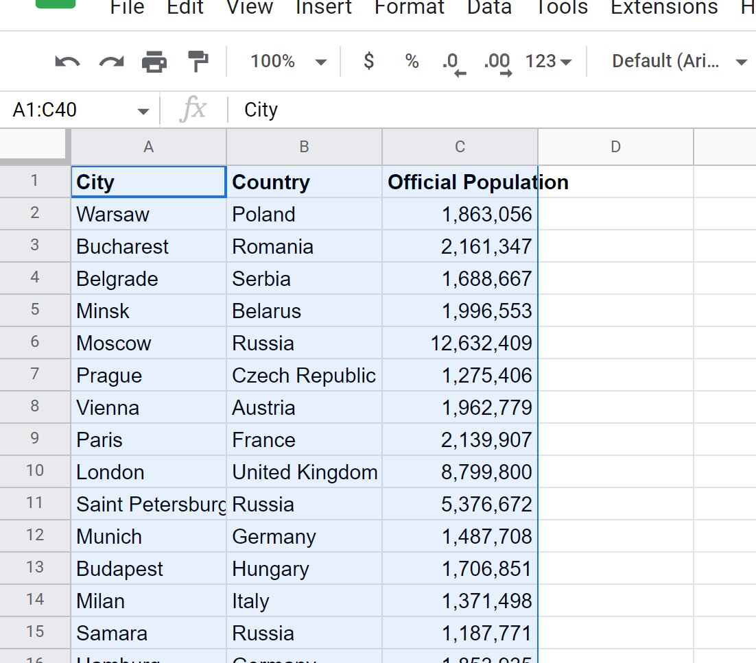
2. Click on the letter of the first column you want to merge. The entire column will be highlighted to indicate that it is selected.
3. Hold down the “Ctrl” key (or “Cmd” key on a Mac) and click on the letter of the second column you want to merge. Both columns will now be selected.
4. If you want to merge more than two columns, continue holding down the “Ctrl” key (or “Cmd” key) and click on the letters of the additional columns you wish to merge.

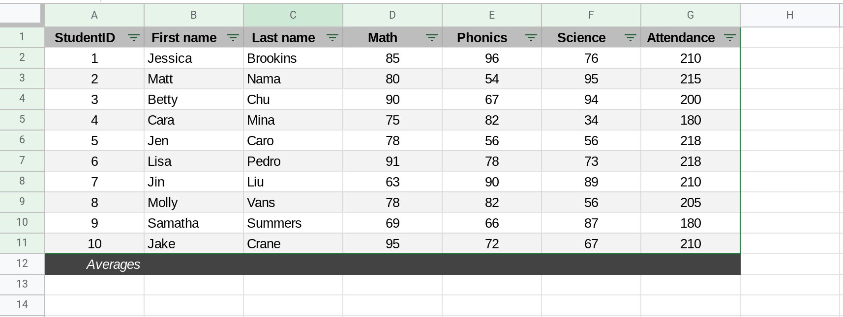
As you select the columns, you will notice that the selected columns are highlighted to distinguish them from the rest of the spreadsheet. This visual feedback ensures that you have selected the correct columns before proceeding with the merge operation.

Now that you have successfully selected the columns you want to merge, you are ready to move on to the next step and perform the merge operation. It’s time to combine the data from the selected columns into a single column for better data management and analysis!

Step 3: Merge the Columns

With the columns selected, you can now proceed to merge them into a single column. Google Sheets provides a simple and straightforward method to accomplish this. Follow the steps below:

1. Right-click on any of the selected column headers.
2. In the context menu that appears, hover over “Merge” and then click on “Merge horizontally”.
3. The selected columns will be merged into a single column, with the content from the first column appearing first, followed by the content from the second column, and so on.

By merging the columns horizontally, you combine the data from the selected columns into a single column, making it easier to work with and analyze. The merged column will be created next to the last selected column, and the original columns will remain intact in the spreadsheet. This ensures that your data is not lost in the merging process, and you can always refer back to the individual columns if needed.

Once the merge operation is completed, you will see the merged column containing the combined data. Take a moment to review the merged column and ensure that the data is merged correctly and in the desired order. If you encounter any issues, you can always undo the merge operation by pressing “Ctrl+Z” (or “Cmd+Z” on a Mac) to revert the changes.

Now that you have successfully merged the selected columns, you can move on to the next step and make any necessary adjustments to the merged column for better readability and data presentation.

Step 4: Adjust the Merged Column

After merging the selected columns, you may need to make some adjustments to the merged column to ensure that the data is properly organized and presented. Here are a few ways you can adjust the merged column in Google Sheets:

• Resize the column: If the merged column is too narrow or wide, you can resize it by hovering over the line between the column headers and dragging it to the desired width.
• Format the data: Depending on the content of the merged column, you may want to apply specific formatting, such as changing the font style, color, or alignment. Use the formatting options in the toolbar to customize the appearance of the merged data.
• Remove duplicates: If the merged column contains duplicate values, you can easily remove them by selecting the merged column, clicking on “Data” in the menu, and choosing “Remove duplicates”. This will ensure that each value appears only once in the merged column.
• Sort the data: If you want to sort the merged column in a specific order, select the merged column, click on “Data” in the menu, and select “Sort sheet by column”. Choose the merged column as the sort column, and select the desired sorting order (ascending or descending).
• Split the merged column: In some cases, you may realize that the merged column needs to be split back into separate columns. To do this, select the merged column, click on “Data” in the menu, and choose “Split text to columns”. Google Sheets will attempt to split the merged column based on common delimiters such as commas or spaces.

By adjusting the merged column, you can customize the appearance and organization of the merged data to suit your specific needs. Take some time to explore the various formatting and manipulation options available in Google Sheets to fine-tune the merged column and optimize it for your data analysis or presentation purposes.

Now that you have made the necessary adjustments to the merged column, you can proceed to repeat the process for additional columns if needed. Follow the next step to merge more columns in Google Sheets.

Step 5: Repeat for Additional Columns

If you have more than two columns that need to be merged in Google Sheets, you can easily repeat the process to merge additional columns. The steps are similar to the previous ones, with a few slight variations. Here’s how you can merge multiple columns:

1. Select the next set of columns that you want to merge. Follow the same process as in Step 2 by clicking on the first column, holding down the “Ctrl” key (or “Cmd” key on a Mac), and clicking on the subsequent columns you wish to merge.
2. Right-click on any of the selected column headers, hover over “Merge,” and then click on “Merge horizontally” in the context menu.
3. The selected additional columns will be merged into the existing merged column, creating a larger merged column that incorporates all of the selected columns.

Repeat this step for any remaining columns that you want to merge. You can merge as many columns as needed, combining the data from each selected column into the merged column. The merged column will continue to expand horizontally to accommodate the merged data.

Remember to adjust the merged column and perform any necessary formatting, resizing, or data manipulation as described in Step 4. This will ensure that the merged column is properly structured and presented after merging multiple columns.

By following this step-by-step process, you can merge multiple columns in Google Sheets and consolidate your data for better analysis and organization. The flexibility of Google Sheets allows you to merge columns effortlessly, saving you time and effort while managing your spreadsheet data effectively.

With the completion of this step, you have successfully merged multiple columns in Google Sheets. Take a moment to review the merged data and make any further adjustments if necessary. Once you are satisfied with the merged columns, you can continue working with your spreadsheet and enjoy the benefits of a more streamlined and consolidated data structure.

Conclusion

Congratulations! You have successfully learned how to merge columns in Google Sheets. This process allows you to combine data from multiple columns into a single column, making it easier to manage, analyze, and present your data effectively.

We started by opening Google Sheets and selecting the columns we wanted to merge. Then, we performed the merge operation by right-clicking on the selected columns and choosing “Merge horizontally”. This merged the columns into a single column, preserving the original data and creating a consolidated view.

After merging the columns, we explored how to adjust the merged column to fit our needs. This included resizing the column, formatting the data, removing duplicates, sorting the data, and even splitting the column back into separate columns if necessary. These adjustments help ensure that the merged data is well-organized and visually appealing.

If you have multiple sets of columns to merge, you can repeat the process for each set by selecting the columns and merging them into the existing merged column. This allows you to merge as many columns as needed, providing a comprehensive view of your data.

Merging columns in Google Sheets is a valuable technique that simplifies data manipulation and enhances data analysis. Whether you are working with complex datasets or simply combining information for easier access, merging columns in Google Sheets can streamline your workflow and improve efficiency.

Now that you have mastered the process of merging columns in Google Sheets, you can confidently apply this technique to your own spreadsheets and enhance your data management capabilities. Experiment with merging columns and discover how it can transform the way you work with your data.

Remember to explore the various formatting options and data manipulation features available in Google Sheets to further customize and enhance your merged columns. With practice and experimentation, you can make the most of Google Sheets’ powerful capabilities and unlock new possibilities in data management.

So go ahead and start merging columns in Google Sheets to take your data organization and analysis to the next level!