Introduction
Google Sheets is a powerful cloud-based spreadsheet tool that offers a wide array of features to help users organize and analyze data. One of the key functionalities provided in Google Sheets is the ability to highlight cells based on certain criteria. This feature allows you to draw attention to specific data points, identify trends, and make your data visually appealing and easy to understand.
With the ability to highlight cells, you can quickly spot important values, identify errors, and create visually appealing reports and dashboards. Whether you’re a data analyst, a project manager, a student, or someone who deals with data regularly, learning how to effectively use highlighting in Google Sheets can significantly boost your productivity and make your data more meaningful.
In this article, we will explore the different ways to highlight cells in Google Sheets, from basic techniques to advanced tips and tricks. We will cover various scenarios, including highlighting single cells, ranges of cells, and using conditional formatting to automate highlighting based on specified criteria. Additionally, we’ll discuss how to remove highlighting when necessary and provide helpful insights on getting the most out of this feature.
By the end of this article, you’ll have a solid understanding of how to effectively use highlighting in Google Sheets and be able to utilize this powerful feature to enhance your data analysis and presentation abilities. So, let’s dive in and explore the world of cell highlighting in Google Sheets.
Why Use Highlighting in Google Sheets
Highlighting cells in Google Sheets serves several important purposes and offers numerous benefits to users. Here are a few compelling reasons why you should incorporate cell highlighting into your data analysis workflow:
1. Visual Emphasis: Highlighting allows you to draw attention to specific cells or data points, making it easier for your audience to quickly identify important information. By visually distinguishing critical data, you can effectively convey your message and ensure that key insights are not overlooked.
2. Data Validation: Highlighting cells based on certain criteria can help validate data and identify errors. By applying conditional formatting rules, you can automatically highlight cells that meet specific conditions, such as values that exceed a threshold or fall within a certain range. This makes it easier to spot inaccuracies and outliers in your data.
3. Trend Identification: Using highlighting, you can spot trends and patterns in your data more easily. By applying conditional formatting rules based on trends, you can highlight cells that show increasing or decreasing values, enabling you to identify growth or decline over a period.
4. Data Comparison: When working with multiple datasets or comparing different scenarios, highlighting cells helps you visually differentiate the data. By applying different colors to cells, you can easily see which values belong to which dataset or scenario, simplifying data comparison and analysis.
5. Presentation Enhancement: Highlighting also plays a crucial role in creating visually appealing reports and presentations. By using a combination of different formats, such as colors, fonts, and borders, you can make your spreadsheets more engaging and professional. This helps in effectively communicating your findings to stakeholders or presenting data in meetings.
These are just a few examples of why highlighting in Google Sheets is a valuable tool for data analysis and presentation. It allows you to emphasize important information, validate data, identify trends, compare datasets, and enhance the visual appeal of your reports and presentations. By incorporating highlighting techniques into your spreadsheet skills, you can take your data analysis to the next level.
How to Highlight Cells in Google Sheets
Highlighting cells in Google Sheets is a straightforward process that can be done using various methods. Let’s explore some of the techniques you can use to highlight cells in Google Sheets:
1. Single Cell Highlighting: To highlight a single cell, you can simply select the cell by clicking on it. Once the cell is selected, you can apply formatting options such as changing the font color, background color, or adding borders using the toolbar at the top of the screen.
2. Range Highlighting: If you want to highlight a range of cells, you can click and drag to select the desired range. Similar to single cell highlighting, you can then apply formatting options to the selected range using the toolbar. This is particularly useful when you want to emphasize a specific section of data or visually separate different sections of your spreadsheet.
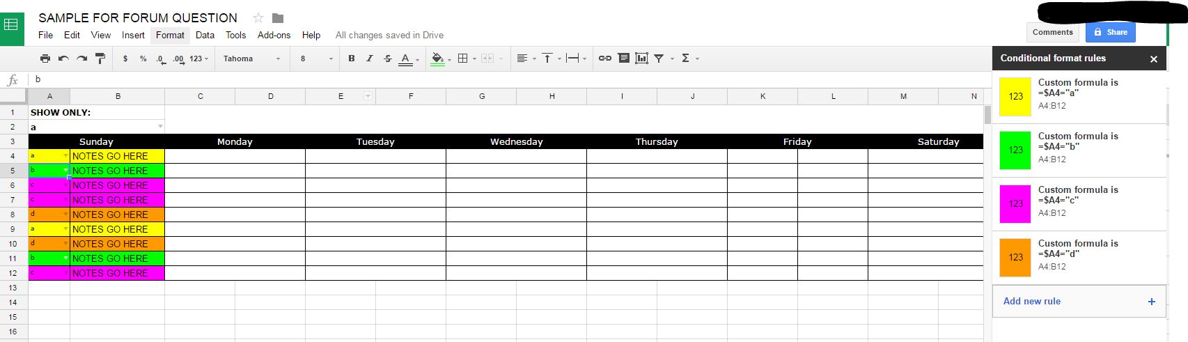
3. Conditional Formatting: Conditional formatting in Google Sheets allows you to automatically highlight cells based on specific conditions or criteria. To access conditional formatting options, go to the “Format” menu, select “Conditional formatting,” and choose the desired rule. For example, you can highlight cells that contain certain text, values within a specific range, or cells that meet custom formulas. Conditional formatting can be a powerful tool for automating highlighting based on dynamic criteria.
4. Data Bars, Color Scales, and Icon Sets: In addition to manually highlighting cells, Google Sheets offers built-in formatting options like data bars, color scales, and icon sets. These options allow you to visually represent data using progressive color gradients, bars, or icons to indicate variations in values. You can access these options under the “Conditional formatting” menu, where you can choose a formatting style that suits your data analysis needs.
5. Custom Formulas: For more advanced scenarios, you can use custom formulas within conditional formatting rules to highlight cells based on your specific requirements. This gives you the flexibility to create complex rules and highlight cells that meet intricate conditions. By utilizing custom formulas, you can fully leverage the power of conditional formatting to highlight cells precisely according to your data analysis needs.
By mastering these techniques, you can effectively highlight cells in Google Sheets and make your data more visually appealing and insightful. Whether you need to emphasize specific values, validate data, or create visually stunning reports, the highlighting features in Google Sheets have got you covered.
Using Conditional Formatting to Highlight Cells
Conditional formatting is a powerful feature in Google Sheets that allows you to automatically highlight cells based on specific conditions. It provides a flexible and efficient way to visually emphasize important data points and make your analysis more effective. Here’s how you can use conditional formatting to highlight cells in Google Sheets:
1. Select the Cells: First, select the cells that you want to apply conditional formatting to. You can choose a single cell, a range of cells, or even an entire column or row.
2. Access Conditional Formatting: Go to the “Format” menu at the top of the screen, then select “Conditional formatting.” This will open the conditional formatting sidebar on the right-hand side of the screen.
3. Choose a Rule: In the conditional formatting sidebar, you will see different rule options. You can choose from pre-defined rules like “Greater than,” “Text contains,” or “Date is before,” or create a custom formula for advanced conditions.
4. Set the Condition: Depending on the rule you choose, you will need to set the condition or value that triggers the formatting. For example, if you choose the “Greater than” rule, you will need to specify the threshold value that, when exceeded, triggers the cell highlighting.
5. Select the Formatting Style: After setting the condition, you can define the formatting style for the highlighted cells. This includes options like font color, background color, borders, or even using icons or data bars. Customize the formatting style according to your preference and visualization needs.
6. Apply the Rule: Once you’ve set the condition and formatting style, click the “Done” button. The formatting rule will be applied to the selected cells, and any cells that meet the specified condition will be automatically highlighted based on the defined formatting style.
You can add multiple conditional formatting rules to the same set of cells, which allows for more complex formatting scenarios. Simply click the “Add another rule” button in the conditional formatting sidebar and repeat the steps above for each additional rule.
Conditional formatting is a dynamic feature in Google Sheets, which means that if the data in the cells changes, the highlighting will automatically update based on the new values. This makes it a valuable tool for data monitoring, trend identification, and error validation.
By utilizing conditional formatting, you can save time, improve data analysis efficiency, and visually highlight critical information in your Google Sheets. Experiment with different conditions and formatting options to find the best combination that suits your data analysis needs.
Highlighting Multiple Cells at Once
In Google Sheets, you can easily highlight multiple cells at once to apply formatting or conditional formatting to a large range of data. This allows for efficient and consistent formatting across a group of cells. Here’s how you can highlight multiple cells simultaneously in Google Sheets:
1. Select a Range of Cells: To highlight multiple cells, simply click and drag your cursor to select the range of cells you want to highlight. You can select a rectangular range or even a non-contiguous set of cells by holding down the Ctrl key (or Command key on a Mac) while clicking on individual cells.
2. Apply Formatting: Once you have selected the desired range of cells, you can apply formatting options such as changing the font color, background color, borders, or using conditional formatting rules to the entire selected range. Any formatting options you choose will be applied to all the selected cells simultaneously.
3. Use the Paint Format Tool: Another efficient way to highlight multiple cells is by using the “Paint format” tool. This tool allows you to copy and apply formatting from a selected cell or range to other cells with a single click. To use the Paint format tool, select a cell or range with the desired formatting, click on the “Paint format” icon in the toolbar, and then click and drag over the cells you want to apply the formatting to.
4. Apply Conditional Formatting: If you want to highlight multiple cells based on specific conditions, you can use conditional formatting. After selecting the range of cells, go to the “Format” menu and choose “Conditional formatting.” Set up the desired rules and formatting styles, and then click “Done.” The conditional formatting will be applied to all the selected cells simultaneously.
Using these methods, you can quickly and efficiently highlight multiple cells in Google Sheets. This is especially useful when you have large datasets or need to apply consistent formatting across a range of cells. By applying formatting or conditional formatting to multiple cells at once, you can save time and ensure consistency in your data analysis and presentation.
Removing Highlighting in Google Sheets
Sometimes, you may need to remove highlighting from cells in Google Sheets to revert them back to their default formatting. Whether you want to remove individual cell formatting or clear all highlighting from a range of cells, Google Sheets provides simple methods to achieve this. Here’s how you can remove highlighting in Google Sheets:
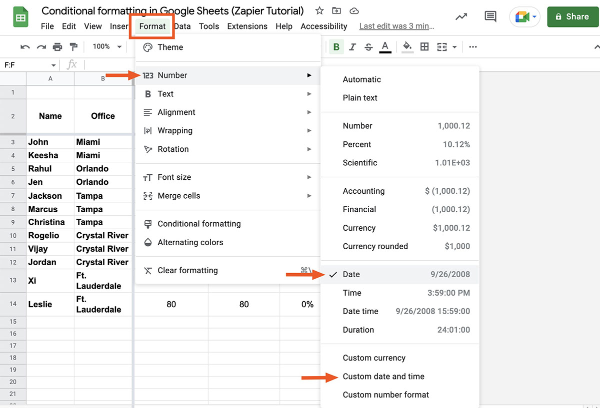
1. Removing Formatting from Individual Cells: To remove formatting from a single cell, you can right-click on the cell and select “Format cells” from the context menu. In the Format cells dialog box, navigate to the “Number” tab and choose the desired format category. Select “Plain text” or any other suitable format to remove any formatting or highlighting from the cell.
2. Clearing Formatting from a Range of Cells: If you want to remove highlighting from a range of cells, select the cells by clicking and dragging or by using the Ctrl (or Command) key while selecting non-contiguous cells. Once selected, right-click on any of the selected cells and choose “Clear formatting” from the context menu. This will remove any formatting, including highlighting, from the selected range of cells.
3. Clearing Conditional Formatting: If you have applied conditional formatting to a range of cells and want to remove it, select the cells, go to the “Format” menu, and choose “Conditional formatting.” In the conditional formatting sidebar, click on the “Clear rules” button at the bottom. This will remove all conditional formatting rules applied to the selected cells.
By using these methods, you can easily remove formatting and highlighting from cells in Google Sheets. Whether you need to remove formatting from individual cells or clear highlighting from a range of cells or conditional formatting rules, Google Sheets provides user-friendly options to revert the cells back to their default formatting.
Don’t forget to double-check your data before removing highlighting to ensure that you don’t accidentally erase any important information. Removing formatting or highlighting is a reversible process, so if needed, you can also reapply formatting and conditional formatting rules as per your requirements.
Advanced Tips and Tricks for Highlighting in Google Sheets
Highlighting cells in Google Sheets can go beyond the basic techniques we’ve covered so far. There are several advanced tips and tricks that can help you take your cell highlighting skills to the next level. Here are some advanced techniques you can try:
1. Use Formulas in Conditional Formatting: Instead of relying solely on pre-defined conditions, you can leverage custom formulas in conditional formatting. This allows you to highlight cells based on complex logic and calculations. For example, you can use formulas to highlight cells that contain specific text, meet multiple conditions, or match specific patterns.
2. Incorporate Data Validation: By combining data validation rules with conditional formatting, you can create sophisticated highlighting scenarios. For instance, you can set up data validation rules to restrict data entry to specific values, and then use conditional formatting to highlight cells that violate those rules. This helps in maintaining data integrity and ensuring consistency.
3. Utilize Advanced Formatting Features: Google Sheets offers advanced formatting options like gradient backgrounds, color scales, and icon sets. These features allow you to visually represent data patterns, trends, or comparisons more effectively. Experiment with different formatting styles to find the one that enhances the clarity and insights of your data.
4. Combine Multiple Formatting Rules: You can apply multiple conditional formatting rules to a range of cells. By using different formatting rules together, you can create more comprehensive highlighting scenarios. For example, you can highlight cells that meet one rule with a specific color, and cells that meet another rule with a different color. This helps in prioritizing and visually categorizing data.
5. Apply Conditional Formatting across Sheets: Conditional formatting can be applied across multiple sheets in a Google Sheets file. This allows you to maintain consistent formatting and highlighting rules across different sheets within the same workbook. By linking formatting rules across sheets, you can ensure coherence and streamline data analysis.
6. Create Heat Maps: Heat maps are a popular visualization technique that uses color gradients to represent data intensity or density. You can create heat maps in Google Sheets by applying color scales using conditional formatting. This helps in visually identifying patterns, trends, or variations in data.
By utilizing these advanced tips and tricks, you can unlock the full potential of highlighting in Google Sheets. Experiment with different techniques, be creative, and tailor the highlighting to your specific data analysis needs. With practice, you’ll be able to produce visually stunning and insightful spreadsheets that make your data come to life.
Summary
Highlighting cells in Google Sheets is a valuable feature that allows you to draw attention to specific information, validate data, identify trends, and create visually appealing reports. In this article, we covered various techniques for highlighting cells in Google Sheets, from basic methods to advanced tips and tricks.
We started by discussing the importance of cell highlighting and how it enhances data analysis and presentation. We then explored how to highlight cells using different methods, including selecting single cells, highlighting ranges, and utilizing conditional formatting.
Conditional formatting is a powerful tool that automates cell highlighting based on specified conditions. We learned how to set up conditional formatting rules and apply them to highlight cells that meet specific criteria. Additionally, we discussed advanced techniques such as using custom formulas, incorporating data validation, and utilizing advanced formatting options like gradients and icon sets.
We also covered how to highlight multiple cells at once to save time and ensure consistency in formatting. Additionally, we learned how to remove highlighting from cells when needed, as well as clear conditional formatting rules.
To conclude, highlighting cells in Google Sheets is a versatile feature that allows you to make your data visually appealing, validate information, and derive insights. By mastering the various techniques and advanced tips covered in this article, you can enhance your data analysis capabilities and create impactful spreadsheets that effectively convey information to your audience.