Introduction
Conditional formatting is a powerful feature in Google Sheets that allows you to dynamically format cells based on certain conditions or criteria. Whether you want to highlight specific values, apply color scales, or add icons to your data, conditional formatting can make your spreadsheet more visually appealing and easier to interpret.
In this article, we will explore the various aspects of conditional formatting in Google Sheets and guide you through the process of applying basic and advanced formatting rules. We will also share some tips and tricks to help you make the most of this feature and enhance your data analysis.
By leveraging the flexibility and versatility of conditional formatting, you can quickly identify trends, outliers, or specific patterns in your data without spending hours manually applying formatting changes. With just a few simple steps, you can create powerful visual cues that highlight key information in your spreadsheet.
Whether you are a data analyst, a student, or a business professional, mastering conditional formatting in Google Sheets will undoubtedly boost both your productivity and the effectiveness of your data analysis. So, let’s dive in and explore the world of conditional formatting in Google Sheets.
Understanding Conditional Formatting in Google Sheets
Conditional formatting is a feature in Google Sheets that allows you to apply formatting to cells based on specific conditions. It helps you highlight important information, spot trends, and make your data more visually appealing and easy to interpret.
With conditional formatting, you can format cells based on their values, the presence of specific text, date ranges, and more. This dynamic formatting feature saves you time and effort by automatically applying formatting rules to your data, eliminating the need for manual formatting.
One of the key benefits of conditional formatting in Google Sheets is the ability to customize the format based on your specific needs. You can choose from a variety of formatting options, including font color, background color, borders, font style, and even the addition of icons.
To apply conditional formatting in Google Sheets, start by selecting the range of cells you want to format. Then, navigate to the “Format” menu and click on “Conditional formatting.” This will open the conditional formatting pane, where you can choose from pre-defined formatting rules or create your own custom rules based on formulas.
Google Sheets provides a range of pre-defined conditional formatting rules to apply to your data. These rules include highlighting cells that contain specific text, numerical values greater or less than a certain threshold, date ranges, or even duplicates. You can select these rules and customize the formatting options to suit your preferences.
If the pre-defined rules don’t meet your requirements, you can create your own custom formulas to define the conditions for formatting. You can use logical operators, functions, and cell references within the formula to apply formatting based on complex conditions. This flexibility allows you to create advanced formatting rules that cater to the specific needs of your data analysis.
As you work with conditional formatting, it’s important to understand that the formatting rules are applied in a hierarchical order. This means that if multiple rules apply to a cell, the formatting rule with the highest priority will be applied. You can manage the order of the rules and their priorities to ensure the desired effects are achieved.
Now that we have a basic understanding of conditional formatting in Google Sheets, let’s explore the process of applying basic and custom formatting rules in the next section.
Applying Basic Conditional Formatting Rules
Applying basic conditional formatting rules in Google Sheets is a straightforward process that allows you to quickly highlight cells based on specific criteria. Let’s delve into the steps to apply these formatting rules to your data.
1. Select the range of cells: Start by selecting the range of cells you want to apply conditional formatting to. You can select a single cell, a range of cells, or even an entire column or row.
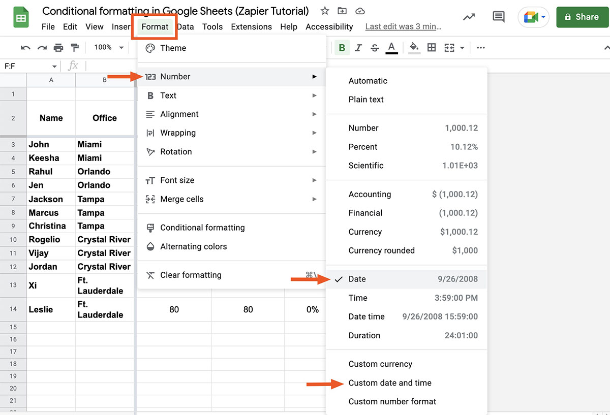
2. Access the conditional formatting options: Navigate to the “Format” menu, click on “Conditional formatting,” and a sidebar will appear on the right side of your screen.
3. Choose the formatting rule: In the conditional formatting sidebar, you will find a variety of pre-defined rules to choose from. These rules include highlighting cells that contain specific text, numerical values greater or less than a certain threshold, date ranges, and more.
4. Customize the rule: Once you have selected a formatting rule, you can customize it based on your preferences. You can choose the formatting style, such as font color, background color, or adding borders. Additionally, you can set the criteria for the rule, such as the value range or specific text to look for.
5. Apply the rule: After customizing the formatting rule, click on the “Done” button, and the formatting will be applied to the selected range of cells. You will immediately see the effects of the rule on your data.
By following these steps, you can quickly apply basic conditional formatting rules to your data in Google Sheets. Experiment with different rules and formatting options to find the best way to highlight and analyze your data effectively.
Remember, you can apply multiple conditional formatting rules to the same range of cells, allowing you to highlight various aspects of your data simultaneously. You can customize the order and priority of these rules to achieve the desired formatting effects.
With basic conditional formatting rules, you can easily identify important values, compare data points, or highlight specific patterns in your spreadsheet. It is a powerful tool that helps you make sense of your data at a glance.
In the next section, we will explore how to use custom formulas to create more advanced conditional formatting rules in Google Sheets.
Using Custom Formulas for Conditional Formatting
While pre-defined rules in Google Sheets provide a range of options for conditional formatting, there are situations where you may need more flexibility and control. This is where custom formulas come into play. By using custom formulas, you can create advanced conditional formatting rules that perfectly suit your data analysis needs.
To use custom formulas for conditional formatting in Google Sheets:
1. Select the range of cells: Start by selecting the range of cells where you want to apply conditional formatting.
2. Access the conditional formatting options: Navigate to the “Format” menu, click on “Conditional formatting,” and a sidebar will appear on the right side of your screen.
3. Choose “Custom formula”: In the conditional formatting sidebar, select “Custom formula” from the “Format cells if” drop-down menu.
4. Write your custom formula: In the textbox below the “Format cells if” drop-down menu, enter your desired formula. This formula should evaluate to either “TRUE” or “FALSE” for each cell in the selected range.
5. Set the formatting style: Customize the formatting style for the cells that meet the conditions specified in the custom formula. You can choose font color, background color, borders, and other formatting options.
6. Apply the rule: After customizing the formatting style, click on the “Done” button to apply the custom formula rule to the selected range of cells.
Custom formulas allow you to apply conditional formatting based on complex conditions that are not covered by the pre-defined formatting rules. You can use logical operators (such as “AND”, “OR”, “NOT”), comparison operators (such as “=”, “<", ">“), functions, and cell references within your formulas.
For example, let’s say you have a range of cells containing test scores, and you want to highlight cells that have a score above a certain threshold. You can use a custom formula like “=B2 > 80” to highlight cells where the value in cell B2 is greater than 80.
By using custom formulas, you can unlock the full potential of conditional formatting in Google Sheets. You can create complex rules that address specific data analysis requirements and highlight patterns or outliers in your data.
Now that we have explored the use of custom formulas for conditional formatting, let’s move on to the next section, where we will discuss working with multiple conditions.
Working with Multiple Conditions
In many cases, you may need to apply conditional formatting based on multiple conditions. Fortunately, Google Sheets allows you to combine multiple conditions to create more complex formatting rules. This enables you to customize your conditional formatting even further and bring out more meaningful insights from your data.
To work with multiple conditions in conditional formatting in Google Sheets, follow these steps:
1. Select the range of cells: Start by selecting the range of cells where you want to apply conditional formatting.
2. Access the conditional formatting options: Navigate to the “Format” menu, click on “Conditional formatting,” and the conditional formatting sidebar will appear on the right side of your screen.
3. Choose “Custom formula” or a pre-defined rule: Depending on the complexity of your conditions, you can either select “Custom formula” if you want to create a custom formula or choose a pre-defined rule that allows for multiple conditions.
4. Write your custom formula or configure the rule: Enter your custom formula or configure the pre-defined rule with multiple conditions. You can use logical operators like “AND” or “OR” to combine conditions within your formula.
5. Set the formatting style: Customize the formatting style for the cells that meet the conditions specified in the formula or pre-defined rule. This includes options like font color, background color, borders, and more.
6. Apply the rule: After customizing the formatting style, click on the “Done” button to apply the rule with multiple conditions to the selected range of cells.
Working with multiple conditions allows you to create more comprehensive formatting rules. For example, you can highlight cells that are both above a certain threshold and belong to a specific category. By combining conditions, you can effectively highlight the most relevant data points in your spreadsheet.
Remember to ensure the proper order and hierarchy of your conditions. The order in which you apply the conditions can influence the formatting results. You can manage the order of the rules in the conditional formatting sidebar to control the priority of each condition.
With the ability to work with multiple conditions, you can effectively customize your conditional formatting to meet the specific needs of your data analysis. Experiment with different combinations of conditions to uncover valuable insights and trends in your spreadsheet.
In the next section, we will discuss how to manage and modify your conditional formatting rules in Google Sheets.
Managing Conditional Formatting Rules
Managing conditional formatting rules in Google Sheets allows you to modify, prioritize, and organize your formatting rules to ensure they best fit your data analysis needs. Let’s explore some key actions you can take to efficiently manage your conditional formatting rules.
1. Edit or modify existing rules: To make changes to an existing formatting rule, navigate to the “Format” menu, click on “Conditional formatting,” and the conditional formatting sidebar will appear. Locate the rule you want to modify and update the formula, formatting style, or range as needed. Click “Done” to apply the changes.
2. Add new rules: If you want to apply additional formatting rules to the same range of cells, click on the “Add another rule” button in the conditional formatting sidebar. This allows you to combine multiple formatting rules and specify different conditions and formatting styles for each rule.
3. Delete rules: To remove a formatting rule, select the rule you want to delete from the list in the conditional formatting sidebar and click on the trash bin icon next to it. This will remove the rule and revert the formatting to the default style.
4. Reorder rules: When working with multiple formatting rules, the order in which you apply the rules can affect the formatting results. To change the order of the rules, use the up and down arrows next to each rule in the conditional formatting sidebar. This allows you to prioritize the rules and ensure they are applied in the desired sequence.
5. Copy and paste rules: To save time when applying similar formatting rules to different ranges or worksheets, you can copy and paste the formatting rules. Simply select the cells with the formatting you want to copy, press “Ctrl+C” or “Cmd+C” to copy, then select the target range or worksheet and press “Ctrl+V” or “Cmd+V” to paste the formatting rules.
By efficiently managing your conditional formatting rules, you can easily update, add, or remove rules to adapt to changing data requirements. Regularly reviewing and revising your rules ensures that the formatting remains useful and relevant to your data analysis.
Additionally, organizing your formatting rules in a logical manner allows you to easily navigate and understand the applied formatting. This is especially important when working with complex spreadsheets that may have numerous conditional formatting rules in use.
Now that we have discussed managing conditional formatting rules, let’s move on to the next section, where we will explore how to clear conditional formatting in Google Sheets.
Clearing Conditional Formatting in Google Sheets
Clearing conditional formatting in Google Sheets allows you to remove all formatting rules applied to a range of cells or an entire worksheet. This can be helpful when you want to start fresh with formatting or when you no longer need the conditional formatting applied to your data.
To clear conditional formatting in Google Sheets, follow these simple steps:
1. Select the range of cells or the entire worksheet: Start by selecting the range of cells where you want to clear the conditional formatting. If you want to clear the formatting applied to the entire worksheet, click on the select all button located at the top-left corner of the spreadsheet (between column A and row 1).
2. Access the conditional formatting options: Navigate to the “Format” menu, click on “Conditional formatting,” and the conditional formatting sidebar will appear on the right side of your screen.
3. Clear the formatting rules: Within the conditional formatting sidebar, click on the “Clear rules” button located at the bottom. This will remove all the conditional formatting rules applied to the selected range or sheet.
4. Confirm the action: A dialog box will appear, asking you to confirm the removal of the conditional formatting rules. Click on “Remove” to proceed with clearing the formatting or click on “Cancel” to cancel the action.
After clearing the conditional formatting, the selected range or worksheet will revert to the default formatting style. This removes any highlighting, color scales, data bars, or icons that were previously applied through the conditional formatting rules.
Clearing conditional formatting is particularly useful when you no longer need the formatting or when you want to remove any formatting conflicts that may have arisen. It provides a clean slate to work with and allows you to implement new formatting rules or apply default formatting to your data.
Remember that clearing conditional formatting is a permanent action, and it cannot be undone. Therefore, proceed with caution and ensure that you have a backup of your data or have saved a copy of the workbook before clearing the formatting.
Now that we have covered how to clear conditional formatting in Google Sheets, let’s move on to the next section, where we will share some tips and tricks for effective conditional formatting.
Tips and Tricks for Effective Conditional Formatting
Conditional formatting in Google Sheets offers a range of possibilities to enhance your data analysis. To make the most out of this feature and create impactful visual displays, consider these tips and tricks:
1. Use color gradients wisely: When applying color scales or color gradients, choose colors that are visually appealing and easily distinguishable. Avoid using colors that may cause confusion or make it difficult to interpret the data. Experiment with different color combinations to find the ones that best represent your data.
2. Combine formatting rules: Utilize multiple formatting rules to highlight different aspects of your data simultaneously. For example, you can use icons to indicate trends, color scales to show variations, and text formatting to draw attention to specific values. This layered approach provides a comprehensive visual representation of your data.
3. Customize icon sets: When using icons for conditional formatting, customize the icon set to align with the context of your data. For example, if you are tracking progress, choose icons that represent different stages or milestones. This helps convey information quickly and intuitively.
4. Format empty cells: If you have empty cells in your dataset, apply conditional formatting to highlight them. This can help you spot missing or incomplete data and ensure the integrity of your analysis.
5. Combine formulas with cell references: Combine custom formulas with cell references to create dynamic formatting rules. By referring to a cell that contains a threshold or a parameter, you can easily update the formatting rule by changing the referenced cell’s value, providing flexibility in your analysis.
6. Use data validation: Pair data validation with conditional formatting to create interactive spreadsheets. You can set up drop-down menus or checkboxes to allow users to select different criteria, which then trigger conditional formatting rules. This enhances the usability and interactivity of your spreadsheet.
7. Test and preview rules: Before applying conditional formatting to a large range of data, try it out on a smaller sample to examine the formatting results. Use the “Preview” feature in the conditional formatting sidebar to assess how your formatting rules apply to different data scenarios.
8. Document your formatting rules: Keep track of your conditional formatting rules by documenting them in a separate sheet or cell comments. This documentation will serve as a reference and help you understand and maintain the formatting clarity when revisiting your spreadsheet later.
By following these tips and implementing them effectively, you can create compelling and informative visual displays in your Google Sheets. The goal is to enhance the readability and insights of your data analysis.
Now that we have covered tips and tricks for effective conditional formatting, let’s conclude this article by summarizing the key takeaways.
Conclusion
Conditional formatting in Google Sheets is a powerful tool that allows you to visually highlight and analyze your data with ease. By applying formatting rules based on specific criteria, you can quickly identify patterns, outliers, and important information in your spreadsheet.
In this article, we explored the fundamentals of conditional formatting, including how to apply basic and custom formatting rules. We also discussed working with multiple conditions, managing and modifying formatting rules, clearing conditional formatting, and shared some tips and tricks for effective formatting.
Remember, conditional formatting is a flexible feature that can be tailored to suit your unique data analysis needs. Whether you’re tracking progress, comparing values, or analyzing trends, conditional formatting can provide valuable insights at a glance.
As you use conditional formatting, keep in mind that readability and visual appeal are crucial. Experiment with different formatting styles, colors, and icon sets to find the best ways to represent and interpret your data. When applying multiple formatting rules, ensure they work together harmoniously to create a clear and meaningful display of your data.
Lastly, stay organized and document your formatting rules for future reference. Regularly review and update your formatting as needed to maintain accuracy and relevance in your data analysis.
With the knowledge and understanding gained from this article, you are well-equipped to leverage the power of conditional formatting in Google Sheets. Start exploring and enhancing your spreadsheets today to unlock valuable insights and make data-driven decisions with confidence.