How To Hide A Row In Google Sheets

Introduction

Google Sheets is a powerful tool for organizing and analyzing data, whether it’s for personal or professional use. One useful feature in Google Sheets is the ability to hide rows, which allows you to temporarily remove specific rows from view without deleting them. This can be helpful when you want to focus on specific data or temporarily hide sensitive information.

In this article, we will guide you through the steps to hide and unhide rows in Google Sheets. Whether you’re a beginner or an experienced user, this simple process can be easily executed in just a few clicks, making it a convenient feature to utilize. So, let’s get started with hiding rows in Google Sheets!

Before we dive into the steps, it’s essential to note that hiding rows in Google Sheets is a formatting feature. This means that although the rows are hidden from view, the data in those rows is still present and will be included in any calculations or functions applied to the sheet. It’s a great way to temporarily declutter your sheet without losing any important data!

Now that you have a clear understanding of the purpose and benefits of hiding rows in Google Sheets, let’s move on to the step-by-step process to hide and unhide rows effortlessly.

Step 1: Open your Google Sheets document

The first step is to open the Google Sheets document where you want to hide a row. If you already have the document open, you can skip to the next step. If not, follow these simple instructions:

1. Launch your web browser and go to sheets.google.com.
2. Sign in to your Google Account if you haven’t already.
3. In the Google Sheets homepage, you will see a list of your saved documents. Click on the document you want to work on, or create a new one by clicking on the “+ Blank” button.
4. Your selected document will open in a new tab, and you will be ready to proceed to the next step.

Ensure you have the necessary access privileges to edit the document so that you can perform the actions required to hide rows. With your Google Sheets document opened, you’re now ready to move on to the next step, where you’ll learn how to select the row(s) you want to hide.

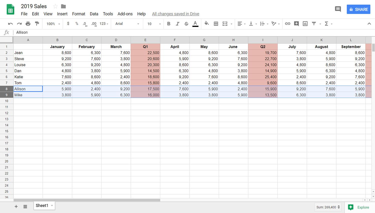
Step 2: Select the row(s) you want to hide

Once you have your Google Sheets document open, you need to select the row or rows that you want to hide. This can be done by following these simple steps:

1. Locate the row number on the left side of your document. Each row will have a corresponding number.
2. Click on the row number of the first row you want to hide. This will select the entire row automatically.
3. If you want to hide multiple rows, you can continue holding down the Ctrl (Windows) or Command (Mac) key and click on the row numbers of the additional rows you want to hide. Each selected row will appear highlighted.
4. Alternatively, if the rows you want to hide are consecutive, you can click on the row number of the first row, hold down the Shift key, and click on the row number of the last row. This will select a range of rows.
5. By following these steps, you can select one or more rows that you wish to hide.

Remember, the selected rows will be hidden, but the data within them will still exist. This means that any formulas, calculations, or references relying on the hidden rows will continue to work properly. Once you have selected the rows you want to hide, you can proceed to the next step to learn how to hide them with a simple right-click.

Step 3: Right click and choose “Hide row”

Now that you have selected the row or rows you want to hide, it’s time to actually hide them from view. Follow these steps to hide the selected row(s) in Google Sheets:

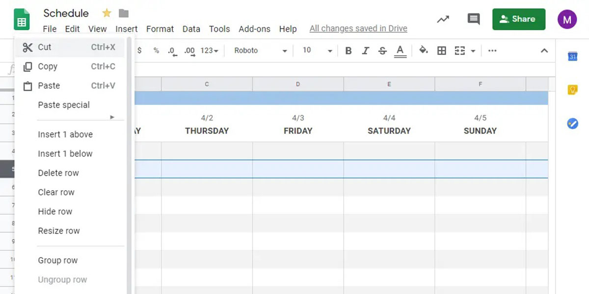
1. With the row(s) selected, right-click on any of the selected row numbers. A drop-down menu will appear.
2. In the drop-down menu, navigate to the “Hide row” option and click on it. This action will instantly hide the selected row(s) from view.

When a row is successfully hidden, you will notice that the row number(s) will disappear from the side of the sheet. The hidden rows will no longer be visible, and your sheet will appear without any gaps or disruptions.

It’s important to reiterate that hiding a row in Google Sheets does not delete the data within it; it simply removes it from view. Therefore, any data, formulas, or functions within the hidden row(s) will still be present and affect the calculations and operations of your sheet.

If you need to hide additional rows, simply repeat the selection and right-click process for each set of rows you wish to hide.

Now that you have successfully hidden the selected row(s), let’s move on to the next step, where you will learn how to verify that the row(s) are indeed hidden.

Step 4: Verify that the row is hidden

After you have hidden a row or multiple rows in Google Sheets, it’s important to verify that they are indeed not visible on the sheet. To check if the row(s) is hidden, follow these simple steps:

1. Look at the side of your sheet where the row numbers are displayed.
2. Scan through the row numbers to locate the range of row numbers that correspond to the rows you hid.
3. If the row numbers of the hidden rows are not visible, it means that the rows are successfully hidden.
4. To further confirm, you can also try scrolling through the sheet and observe that there are no visible gaps or breaks in the data.

Additionally, if you need to refer to any data within the hidden rows, you can still access and modify it using formulas or by unhiding the rows. However, remember that any calculations or operations that include the hidden row(s) will still take them into account.

Verifying that the rows are hidden ensures that you can confidently proceed with your analysis or data manipulation without any distractions. If you need to unhide a hidden row, the next step will guide you through the process.

Step 5: Unhide a hidden row if needed

If you need to make a hidden row visible again in your Google Sheets document, you can easily unhide it using the following steps:

1. Locate the row numbers on the side of your sheet.
2. If there is a hidden row, you will notice a small gap or break in the sequence of row numbers.
3. To unhide a single row, right-click on the row number before and after the hidden row.
4. In the right-click menu, choose the “Unhide row” option, and the hidden row will instantly become visible again.
5. If you have multiple hidden rows consecutively, you can select the row numbers before and after the hidden rows and unhide them using the same process.

Once a hidden row is unhidden, the row number will reappear on the side of the sheet, and the data within it will be visible once again.

Remember that unhiding a row in Google Sheets does not affect the data contained within it. Any existing formulas or calculations that rely on the unhidden row will continue to function as expected.

By following these steps, you can effortlessly unhide any hidden rows that you may need to access or work with in your Google Sheets document.

Now that you have learned how to hide and unhide rows in Google Sheets, you have gained a valuable skill that can help you organize and manipulate your data effectively. Whether it’s for simplifying complex spreadsheets or temporarily hiding sensitive information, this feature provides flexibility and convenience.

Conclusion

Google Sheets offers a simple yet powerful way to hide and unhide rows, allowing you to customize your view and focus on specific data without deleting any important information. By following the steps outlined in this guide, you can easily hide rows in your Google Sheets document to declutter your view, protect sensitive information, or highlight relevant data.

Remember, hiding a row in Google Sheets is a formatting feature, meaning the data within the hidden row still exists and will be included in any calculations or functions applied to the sheet. This ensures the integrity of your data analysis and allows for flexibility in organizing and manipulating your spreadsheet.

Should you need to unhide a row, the process is just as straightforward. Unhiding a row allows you to easily access the data within it while maintaining the interconnectedness of your formulas and calculations.

Utilizing the ability to hide and unhide rows in Google Sheets empowers you to take control of your spreadsheet and present the information in a way that best suits your needs. The flexibility and convenience provided by this feature make it a valuable tool for data analysis, project management, financial tracking, and much more.

Now that you are equipped with the knowledge of how to hide and unhide rows in Google Sheets, you can enhance your productivity and efficiency when working with large amounts of data. Experiment with this feature and explore its possibilities to unlock new ways of organizing and visualizing your data in Google Sheets.