How Do You Unhide Rows In Google Sheets

Introduction

Google Sheets is a powerful tool for organizing and analyzing data. With its vast array of features and functions, it allows users to manipulate data in various ways to suit their needs. One common task in Google Sheets is hiding and unhiding rows, which can be particularly useful when working with large datasets or when wanting to focus on specific sections of a spreadsheet.

In this article, we will explore different methods to unhide rows in Google Sheets. Whether you accidentally hid some rows or intentionally hid them and now need to bring them back into view, these methods will help you easily navigate through your spreadsheet and regain access to the hidden rows.

Before we dive into the different methods, it’s important to note that rows can be hidden in Google Sheets for several reasons. It could be because you hid them manually using the context menu, keyboard shortcuts, or the options menu. Alternatively, certain functions or tools, such as filters or find and replace, can also hide rows based on specific criteria.

Now, let’s explore the various methods available to unhide rows in Google Sheets, ensuring that you have the necessary knowledge to work efficiently with your data.

Method 1: Using the Menu

One of the easiest ways to unhide rows in Google Sheets is by using the menu. This method is straightforward and convenient, making it suitable for users who prefer a more visual approach to spreadsheet navigation.

Here’s how you can unhide rows using the menu:

1. Open your Google Sheets document.
2. Select the range of rows that contain the hidden rows. You can do this by clicking and dragging your mouse over the row numbers, or by using the Shift key to select multiple rows.
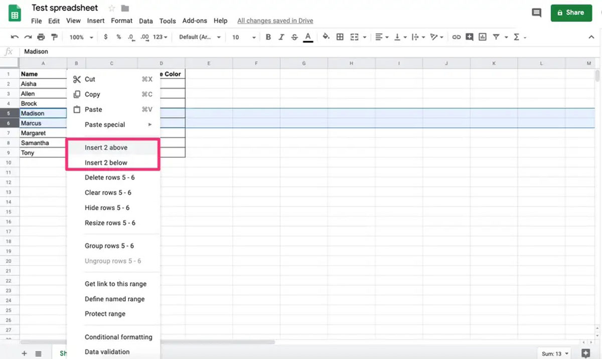
3. Right-click on the selected rows to open the context menu.
4. In the context menu, hover over the “Row” option, and then select “Unhide row” from the submenu.
5. Voila! The hidden rows will now be visible and integrated back into the spreadsheet.

By following these simple steps, you can easily unhide rows using the menu in Google Sheets. This method allows you to interact directly with the spreadsheet interface, making it an intuitive solution for users of all levels of expertise.

Now that you know how to use the menu to unhide rows, let’s move on to the next method, which involves using a convenient keyboard shortcut.

Method 2: Using the Shortcut Key

If you’re someone who prefers using keyboard shortcuts to navigate through Google Sheets, this method is for you. By memorizing a simple shortcut key combination, you can quickly unhide rows without having to rely on the mouse or menu options.

Here’s how you can unhide rows using the shortcut key:

1. Open your Google Sheets document.
2. Select the range of rows that contain the hidden rows. You can do this by clicking and dragging your mouse over the row numbers, or by using the Shift key to select multiple rows.
3. Press Ctrl + Shift + 9 on Windows or Command + Shift + 9 on Mac.

That’s it! The hidden rows will now be visible, and you can continue working with them as needed.

Using the shortcut key provides a swift and efficient method to unhide rows in Google Sheets, especially for users who prefer to keep their hands on the keyboard while working. By utilizing this shortcut, you can save time and streamline your workflow.

Now that you’re familiar with the shortcut key method, let’s explore another option available in the options menu.

Method 3: Using the Options Menu

The options menu in Google Sheets provides a range of functionalities that can make navigating and managing your spreadsheet easier. Unhiding rows is one of the features available in this menu, offering another method to quickly reveal hidden rows.

Here’s how you can unhide rows using the options menu:

1. Open your Google Sheets document.
2. Select the range of rows that contain the hidden rows. You can do this by clicking and dragging your mouse over the row numbers, or by using the Shift key to select multiple rows.
3. Go to the top menu and click on “Format”.
4. In the “Format” menu, hover over the “Rows” option, and then select “Unhide rows” from the dropdown.

Once you click on “Unhide rows,” the hidden rows within the selected range will become visible again.

Using the options menu to unhide rows provides an alternative approach for users who prefer utilizing menu options. This method offers a more comprehensive set of formatting options and allows you to access additional features beyond just unhiding rows.

Now that you’re familiar with the options menu method, let’s move on to another technique, using the Find and Replace tool.

Method 4: Using the Find and Replace Tool

The Find and Replace tool in Google Sheets is a powerful feature that allows you to search for specific values or criteria within your spreadsheet and replace them with new values. Interestingly, this tool can also be used to uncover hidden rows based on specific search criteria.

Here’s how you can unhide rows using the Find and Replace tool:

1. Open your Google Sheets document.
2. Click on the magnifying glass icon in the toolbar or press Ctrl + F on Windows or Command + F on Mac to open the Find and Replace tool.
3. In the search bar, enter a value or criteria that is unique to the hidden rows you want to unhide.
4. Click on the “Find” button or press Enter to start the search process.
5. Once the hidden rows are highlighted as search results, click on the “Replace all” button to unhide them.

Using the Find and Replace tool to unhide rows is an innovative method that takes advantage of the search functionality within Google Sheets. This feature allows you to unhide rows based on specific search criteria, making it useful when you want to selectively reveal specific rows in your spreadsheet.

Now that you’re familiar with using the Find and Replace tool to unhide rows, let’s explore the final method in our repertoire – the Filter tool.

Method 5: Using the Filter Tool

The Filter tool in Google Sheets allows you to sort and filter data based on specific criteria, helping you to focus on relevant information within your spreadsheet. Interestingly, the Filter tool can also be used to reveal hidden rows by manipulating the filtering settings.

Here’s how you can unhide rows using the Filter tool:

1. Open your Google Sheets document.
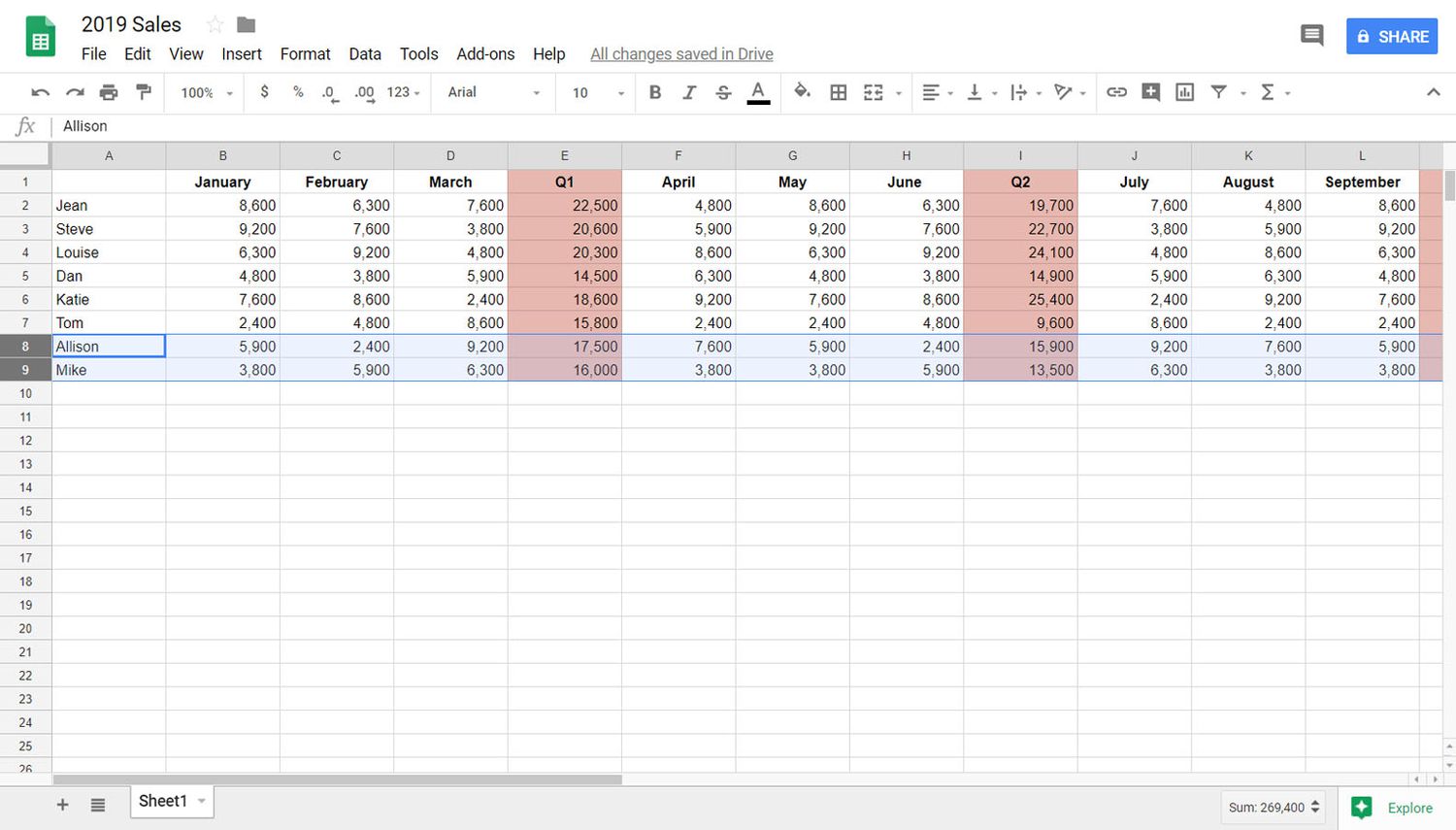
2. Select the entire data range, including any hidden rows, or click on a single cell within the data range.
3. In the top menu, click on “Data”.
4. Select “Filter” from the dropdown menu to activate the Filter tool.
5. In the column header of the hidden rows, click on the filter dropdown arrow.
6. In the filter options, uncheck the box that corresponds to the criteria causing the row to be hidden.

Once you uncheck the box, the hidden rows will be revealed again, as they no longer meet the filtering criteria.

Using the Filter tool to unhide rows provides a dynamic and customizable method of revealing hidden data. This method allows you to unhide rows selectively based on specific criteria, offering flexibility and control over your data visualization.

Now that you’re familiar with using the Filter tool to unhide rows, you’ve discovered five different methods to uncover hidden rows in Google Sheets. Each method provides a unique approach to suit different preferences and workflows. Whether you prefer using the menu, keyboard shortcuts, options menu, Find and Replace tool, or the Filter tool, you now have a plethora of options to unhide rows in your Google Sheets spreadsheet.

Conclusion

Unhiding rows in Google Sheets is a common task that can help you effectively organize and analyze your data. In this article, we explored five different methods to unhide rows: using the menu, shortcut key, options menu, Find and Replace tool, and Filter tool. Each method offers its own advantages and caters to different user preferences.

The menu method provides a visual approach to unhiding rows, allowing users to navigate through the interface intuitively. The shortcut key method is ideal for those who prefer quick keyboard shortcuts to access features. The options menu method offers a comprehensive range of formatting options in addition to unhiding rows. The Find and Replace tool enables users to uncover hidden rows based on specific search criteria. Lastly, the Filter tool provides a dynamic approach to selectively reveal rows based on filtering settings.

By familiarizing yourself with these methods, you can efficiently navigate through your data and bring hidden rows back into view, making your spreadsheet manipulation more seamless and effective.

Remember that the choice of method depends on your personal preferences and the specific requirements of your data analysis. Experiment with each method and find the one that suits your needs best.

With the knowledge gained from this article, you are now equipped to confidently unhide rows in Google Sheets and enhance your data management capabilities in the application.

So go ahead and utilize these methods to effortlessly navigate and manipulate your spreadsheets, unlocking the full potential of Google Sheets for your data analysis needs!