Introduction
Welcome to the fascinating world of machine learning algorithms! With the rapid advancement of technology, the field of machine learning has gained significant attention and is revolutionizing various aspects of our lives. From predicting customer behavior to diagnosing medical conditions, machine learning algorithms enable computers to learn from data and make insightful predictions.
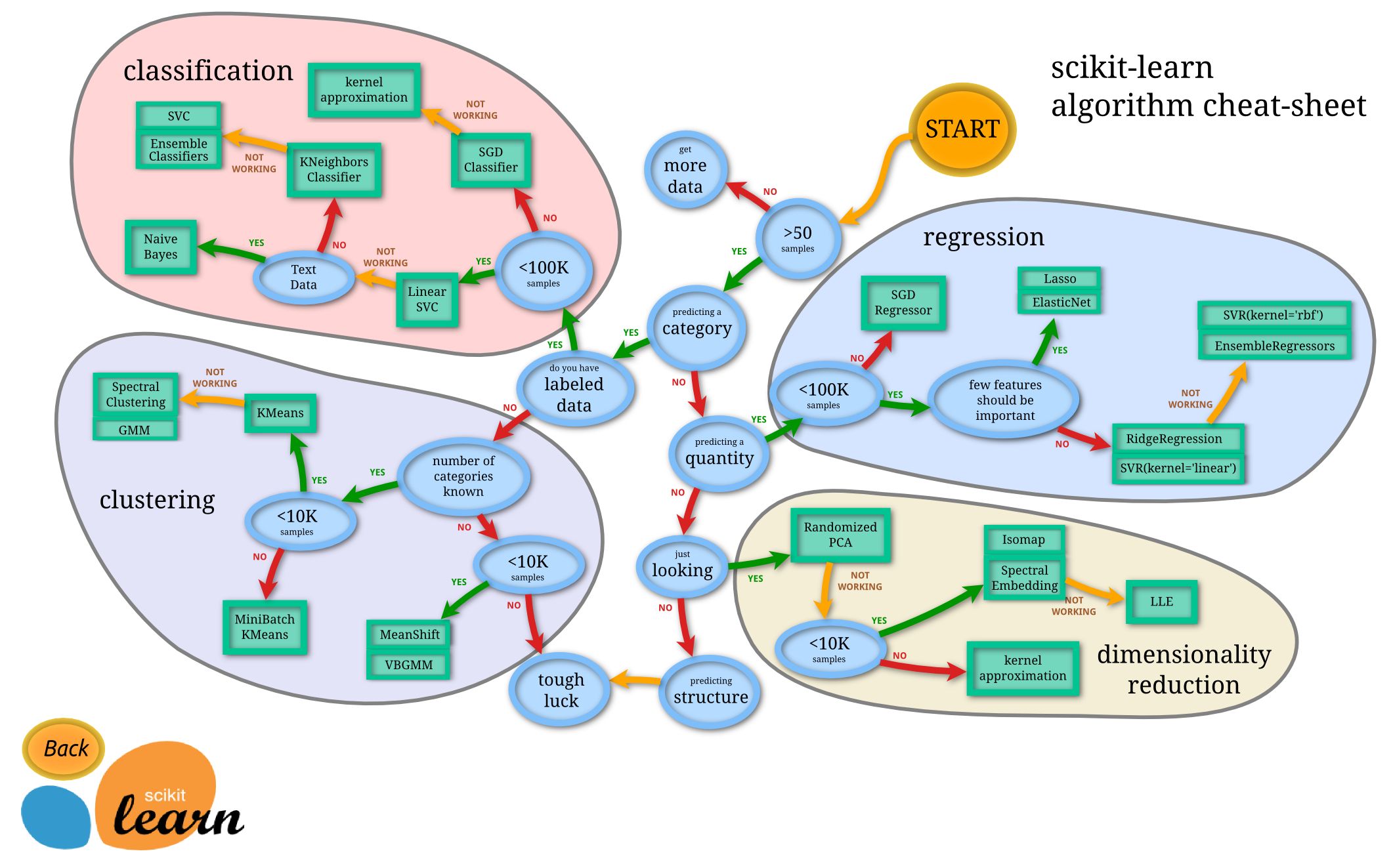
This article aims to provide an overview of different machine learning algorithms and guide you in understanding when to use each one. It is important to note that the choice of algorithm depends on the nature of the problem you are trying to solve, the type of data you have, and the desired outcome.
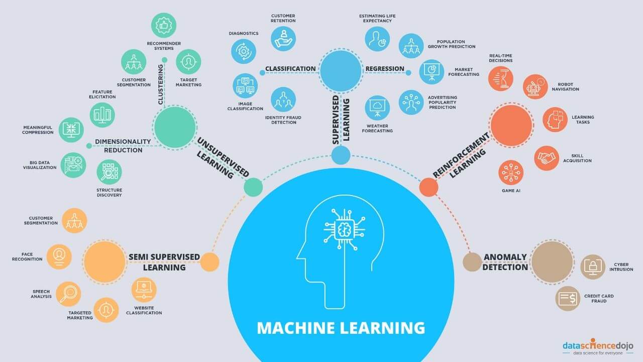
Machine learning algorithms can be broadly categorized into supervised learning, unsupervised learning, and deep learning. Supervised learning algorithms are used when there is a labeled dataset, meaning each data point is already assigned a category or a class. Unsupervised learning algorithms, on the other hand, are used when there is no predefined label for the data. Deep learning algorithms are a subset of neural networks that are capable of learning complex patterns.
Throughout this article, we will explore various machine learning algorithms, including decision trees, random forests, naive Bayes, logistic regression, support vector machines (SVM), k-nearest neighbors (KNN), k-means clustering, principal component analysis (PCA), and deep learning. Each algorithm has its strengths and weaknesses, and understanding their nuances will empower you to select the appropriate one for your specific task.
As we delve into each algorithm, keep in mind that this article serves as a general guide. It is crucial to thoroughly analyze your data, consult domain experts, and conduct experiments to determine the most suitable algorithm for your particular use case.
Now, let’s embark on this exciting journey of exploring machine learning algorithms and discover when to use each one!
Decision Trees
Decision trees are one of the simplest yet powerful machine learning algorithms. They are primarily used for classification tasks but can also be applied to regression problems. As the name suggests, decision trees mimic the decision-making process by creating a tree-like model of decisions and their possible consequences.
Decision trees progressively split the dataset into subsets based on different attributes, aiming to maximize the information gain at each step. At the root of the tree, the algorithm selects the attribute that provides the most significant division of the data. It continues to split the data at each subsequent node until it reaches a leaf node, which represents the final decision or prediction.
One of the key advantages of decision trees is their interpretability. It is easy to visualize and understand how decisions are made and what attributes play a crucial role in the classification. Furthermore, decision trees can handle both numerical and categorical data, making them versatile for a wide range of applications.
However, decision trees are prone to overfitting, especially when dealing with complex datasets. Overfitting occurs when the tree becomes too specific to the training data, leading to poor generalization on unseen data. To mitigate overfitting, techniques like pruning, setting a maximum depth, and implementing regularization methods can be used.
Decision trees are commonly used in various domains, including finance, healthcare, and customer segmentation. For instance, in fraud detection, decision trees can effectively classify transactions as fraudulent or legitimate based on specific features like transaction amount, account age, and transaction history.
To summarize, decision trees are an intuitive and interpretable algorithm that can handle both categorical and numerical data. They are suitable for classification tasks and can be effective in domains where interpretability is crucial. However, caution should be taken to avoid overfitting by applying appropriate regularization techniques.
Random Forests
Random forests are an ensemble learning method that combines multiple decision trees to produce more accurate and robust predictions. This algorithm is particularly effective in handling complex datasets and reducing overfitting, making it a popular choice among data scientists.
The random forest algorithm works by creating a collection of decision trees, each trained on a random subset of the original dataset. These decision trees are then combined to make predictions by majority voting or averaging. The randomness in the training process, such as random selection of features and random sampling of data, helps to introduce diversity into the ensemble, leading to improved generalization performance.
One of the strengths of random forests is that they can handle both classification and regression tasks. In classification problems, random forests provide probabilistic predictions, indicating the confidence of each class label. In regression problems, the algorithm outputs the mean or median prediction of the ensemble.
Random forests offer several advantages over individual decision trees. They are robust against noisy and missing data, making them suitable for real-world datasets. Additionally, random forests are less prone to overfitting due to the ensemble nature of the algorithm, which combines the predictions of multiple trees.
Random forests also provide measures of feature importance, allowing data scientists to identify the most relevant features for prediction. This information can be valuable for feature selection and understanding the underlying patterns in the data.
Random forests are widely used in various domains, including finance, healthcare, and image classification. For example, in the healthcare field, random forests can be employed to predict the likelihood of a patient developing a certain disease based on their medical history, lifestyle factors, and genetic markers.
In summary, random forests are a powerful ensemble learning algorithm that combines multiple decision trees to achieve high prediction accuracy and handle complex datasets. They are robust against noise and missing data, provide measures of feature importance, and are well-suited for both classification and regression tasks.
Naive Bayes
Naive Bayes is a simple yet effective machine learning algorithm based on the Bayes’ theorem. Despite its simplicity, it has shown remarkable performance in many text classification and sentiment analysis tasks.
The algorithm assumes that all features in the dataset are independent of each other, hence the term “naive.” This assumption simplifies the computation but may not hold true in some real-world scenarios. Nevertheless, Naive Bayes can still deliver accurate results, especially when applied to large and high-dimensional datasets.
The Naive Bayes algorithm uses probability and statistics to make predictions. It calculates the probability of each class given the input features and chooses the class with the highest probability as the prediction. To facilitate this, the algorithm computes the prior probability of each class and the likelihood of the input features given each class.
One of the advantages of Naive Bayes is its efficiency in training and prediction. It requires a small amount of training data, and the computational complexity is low compared to more complex algorithms. Naive Bayes is also known to handle irrelevant features well, making it resilient to noisy or irrelevant data.
However, the Naive Bayes algorithm’s independence assumption can limit its accuracy in certain cases. If there are strong dependencies between features, the algorithm may underestimate the interrelationships, leading to suboptimal predictions. Additionally, Naive Bayes is not suitable for tasks that require complex decision boundaries.
Naive Bayes is commonly used in text classification problems, such as email spam filtering, sentiment analysis, and document categorization. For example, in sentiment analysis, the algorithm can classify text as positive, negative, or neutral based on word frequencies and probabilistic calculations.
In summary, Naive Bayes is a straightforward algorithm that leverages probability and statistics to make predictions. It is efficient, handles irrelevant features well, and performs particularly well in text classification tasks. However, its assumption of independence between features may limit its accuracy in certain cases.
Logistic Regression
Logistic regression is a popular machine learning algorithm used for binary classification tasks. Despite its name, logistic regression is actually a classification algorithm rather than a regression algorithm. It is widely adopted in various domains due to its simplicity, interpretability, and robustness.
The logistic regression algorithm models the relationship between the input features and the probability of belonging to a particular class. It utilizes the logistic function, also known as the sigmoid function, to transform the linear combination of input features into a probability value between 0 and 1. This allows for easy interpretation and decision-making.
One of the key advantages of logistic regression is its interpretability. The algorithm assigns weights to each input feature, indicating their influence on the prediction. These weights can provide insights into which features are more important in determining the class of the input data.
Logistic regression also handles noisy data well, making it suitable for real-world applications where the data may be imperfect. It is also less prone to overfitting compared to more complex algorithms, making it suitable for datasets with limited training examples.
However, logistic regression has some limitations. It assumes that the relationship between the input features and the log-odds of the target variable is linear. If the relationship is highly nonlinear, logistic regression may not capture it accurately. Additionally, logistic regression is primarily designed for binary classification and may not perform as well in situations with multiple classes.
Logistic regression finds application in various fields, such as medical diagnosis, credit scoring, and customer churn prediction. For example, in medical diagnosis, logistic regression can be used to predict the likelihood of a patient having a certain disease based on their symptoms and medical history.
In summary, logistic regression is a simple yet powerful algorithm for binary classification tasks. It offers interpretability, handles noisy data well, and is less prone to overfitting. While it assumes a linear relationship between features and the log-odds of the target variable, it finds wide use in various domains.
Support Vector Machines (SVM)
Support Vector Machines, commonly known as SVM, is a popular machine learning algorithm used for both classification and regression tasks. It is particularly effective in scenarios with complex decision boundaries and high-dimensional data.
SVM works by finding the optimal hyperplane that separates the data points of different classes with the largest margin. The hyperplane is chosen in such a way that it maximizes the distance between the nearest data points of each class, known as support vectors. By doing so, SVM aims to achieve the best possible generalization performance on unseen data.
SVM can handle both linearly separable and non-linearly separable datasets through the use of kernel functions. Kernel functions transform the input data into higher-dimensional feature spaces, enabling SVM to find non-linear decision boundaries. Popular kernel functions include linear, polynomial, radial basis function (RBF), and sigmoid.
One of the key advantages of SVM is its ability to handle high-dimensional data effectively. SVM can handle datasets with a large number of features without being affected by the “curse of dimensionality.” It also provides control over the classifier’s margin and flexibility through the use of hyperparameters, allowing fine-tuning to achieve optimal performance.
SVMs are known for their robustness against noise in the data. By maximizing the margin between classes, the algorithm tends to be less affected by outliers and noisy data points, resulting in more reliable predictions.
However, SVMs can be sensitive to the choice of hyperparameters, and finding the optimal values can be computationally expensive for large datasets. Additionally, SVMs may struggle with datasets that have overlapping classes or imbalanced class distributions. In such cases, careful preprocessing or the use of alternative algorithms might be necessary.
SVMs are widely used in various domains, including text classification, image recognition, and bioinformatics. For example, in text classification, SVM can classify documents into different categories based on their content, allowing for efficient document organization and retrieval.
In summary, Support Vector Machines (SVM) are powerful algorithms that can effectively handle high-dimensional data and complex decision boundaries. They are robust against noise and provide control over the classifier’s margin through hyperparameters. While sensitive to hyperparameter choices and potentially challenging with overlapping classes, SVMs find applications in numerous domains.
K-Nearest Neighbors (KNN)
K-Nearest Neighbors (KNN) is a simple and intuitive machine learning algorithm that can be used for both classification and regression tasks. It is known as a non-parametric algorithm because it does not make any assumptions about the underlying data distribution.
The KNN algorithm works by finding the K nearest neighbors to a given data point based on a distance metric, such as Euclidean distance or Manhattan distance. The class or value of the new data point is then determined by majority voting in the case of classification or averaging in the case of regression.
KNN is a lazy learning algorithm, meaning it does not require a training phase. Instead, it stores all the input data points and performs computations at the time of prediction. While this can make the prediction process slower compared to other algorithms, it allows KNN to adapt easily to changes in the training data.
One of the advantages of KNN is its simplicity. It is easy to implement and understand, making it a popular choice for beginners and quick prototyping. KNN also retains all the training data, which can be useful in identifying outliers or anomalies in the dataset.
However, KNN has some limitations. The algorithm can be sensitive to the choice of the number of neighbors, K. If K is too small, the algorithm may be influenced by noise or outliers, while if K is too large, it may not capture local patterns effectively. Additionally, KNN suffers from the curse of dimensionality, where the algorithm’s performance decreases as the number of features increases.
KNN finds applications in recommendation systems, image recognition, and anomaly detection. For example, in recommendation systems, KNN can identify similar users or items based on their shared features, enabling personalized recommendations for users.
In summary, K-Nearest Neighbors (KNN) is a simple and versatile algorithm that can handle classification and regression tasks. It is easy to understand, retains all the training data, and adapts well to changes. However, the choice of the number of neighbors and the curse of dimensionality should be considered when applying KNN to a particular problem.
K-Means Clustering
K-Means Clustering is a widely used unsupervised machine learning algorithm that partitions data into K clusters based on their similarity. It is a simple and efficient algorithm that works well on large datasets and is commonly applied in various fields, including image segmentation, customer segmentation, and anomaly detection.
The K-Means algorithm works by iteratively assigning data points to clusters and then updating the cluster centers. Initially, K cluster centers are randomly selected from the data points, and each data point is assigned to the nearest cluster based on a distance metric, often Euclidean distance. After the initial assignment, the cluster centers are updated by recalculating the mean of each cluster’s data points. This process continues until convergence is reached, and the cluster assignments stabilize.
The objective of K-Means clustering is to minimize the within-cluster sum of squares, also known as the inertia or distortion. This metric measures the distance between each data point and the centroid of its assigned cluster. By minimizing the inertia, K-Means ensures that data points within the same cluster are more similar to each other than to data points in other clusters.
K-Means clustering has several advantages. It is a relatively fast algorithm and can handle large datasets efficiently. It is also straightforward to implement and allows for easy interpretation and visualization of the results. Additionally, K-Means can be used as a preprocessing step for tasks such as outlier detection or as a feature engineering tool.
However, K-Means clustering has some limitations. It requires the number of clusters, K, to be specified in advance, which can be challenging if prior knowledge of the dataset is limited. The algorithm is also sensitive to the initial choice of cluster centers and may converge to suboptimal solutions. Care should be taken to repeat the algorithm multiple times with different initializations to ensure robustness.
K-Means clustering finds applications in a wide range of domains. In image segmentation, K-Means can partition an image into distinct regions based on pixel similarities, enabling object identification and image analysis. In customer segmentation, K-Means can group customers with similar characteristics, helping businesses target specific customer segments with personalized marketing strategies.
In summary, K-Means Clustering is a widely used unsupervised learning algorithm that partitions data into K clusters. It is efficient, easy to implement, and allows for interpretation and visualization of results. Care should be taken in choosing the number of clusters and initializing the cluster centers to ensure optimal performance.
Principal Component Analysis (PCA)
Principal Component Analysis (PCA) is a dimensionality reduction technique commonly used in machine learning and data analysis. It helps to identify patterns and reduce the complexity of high-dimensional datasets by transforming them into a lower-dimensional space while preserving the most important information.
The goal of PCA is to find a set of new variables, called principal components, that capture the maximum amount of variance in the original data. These principal components are linear combinations of the original features and are orthogonal to each other. The first principal component accounts for the most variance in the data, followed by the second component, and so on.
By reducing the dimensionality of the data, PCA can simplify the analysis and visualization of complex datasets. It can also help to remove noise and redundancy, leading to more efficient and accurate models in subsequent analyses.
The PCA algorithm computes the principal components by performing eigenvalue decomposition or singular value decomposition on the covariance matrix or the correlation matrix of the data. The eigenvalues indicate the amount of variance explained by each principal component, while the eigenvectors correspond to the direction of the component in the original feature space.
PCA is commonly used for data preprocessing, feature extraction, and visualization. It has applications in various fields, including image processing, genetics, and finance. For example, in image processing, PCA can be used to reduce the dimensionality of image data while preserving its most salient features, making it easier to classify and analyze images.
It is important to note that PCA assumes linearity and may not be suitable for datasets with complex nonlinear relationships. In such cases, other non-linear dimensionality reduction techniques, such as t-SNE or autoencoders, may be more appropriate.
In summary, Principal Component Analysis (PCA) is a dimensionality reduction technique used to transform high-dimensional data into a lower-dimensional space while preserving important information. It simplifies data analysis, removes noise and redundancy, and aids in visualization. However, it assumes linearity and may not be suitable for datasets with complex nonlinear relationships.
Deep Learning
Deep Learning is a subset of machine learning that focuses on training artificial neural networks to learn and make predictions on complex patterns and large amounts of data. It is inspired by the structure and functioning of the human brain, with multiple layers of interconnected artificial neurons called neural networks.
Deep Learning has gained significant attention and has achieved remarkable success in various fields, such as image recognition, natural language processing, and speech recognition. It has pushed the boundaries of what is possible in terms of accuracy and performance on challenging tasks.
One of the key advantages of Deep Learning is its ability to automatically learn hierarchical representations from raw or high-dimensional data. With each layer in the neural network, the system becomes capable of learning increasingly abstract and complex features. This allows Deep Learning models to extract meaningful patterns and features that may not be easily discernible to humans.
Deep Learning relies on large amounts of labeled data to train the neural networks effectively. It employs powerful optimization algorithms, such as stochastic gradient descent, to iteratively adjust the network’s weights and biases to minimize the prediction error. Additionally, advancements in hardware, such as Graphics Processing Units (GPUs) and specialized chips like Tensor Processing Units (TPUs), have accelerated the training process of deep neural networks.
One of the challenges of Deep Learning is the potential for overfitting, especially when training with limited data. Techniques such as regularization and dropout are commonly used to mitigate this issue and improve generalization performance of the models. Additionally, the interpretability of Deep Learning models can be a concern, as the complexity of the networks makes it difficult to understand the underlying decision-making process.
Deep Learning has numerous applications in various domains. In computer vision, deep neural networks have enabled breakthroughs in object detection, image segmentation, and facial recognition. In natural language processing, deep learning models have revolutionized machine translation, sentiment analysis, and speech recognition.
In summary, Deep Learning is a subset of machine learning that leverages artificial neural networks to learn complex patterns and make predictions on large amounts of data. It excels in tasks that require hierarchical representations and has achieved remarkable success in computer vision, natural language processing, and speech recognition. While overfitting and interpretability can pose challenges, deep learning has transformed the field of AI and continues to drive innovation and advancements.
Conclusion
Machine learning algorithms offer powerful tools for analyzing data, making predictions, and uncovering patterns in complex datasets. In this article, we have explored several widely used algorithms, including decision trees, random forests, naive Bayes, logistic regression, support vector machines (SVM), k-nearest neighbors (KNN), k-means clustering, principal component analysis (PCA), and deep learning.
Each algorithm has its own strengths and limitations, and understanding when to use each one is crucial for achieving successful results. Decision trees provide interpretability and can handle both categorical and numerical data. Random forests improve upon decision trees by reducing overfitting and providing measures of feature importance.
Naive Bayes is a simple yet effective algorithm for text classification and sentiment analysis, while logistic regression is a popular choice for binary classification tasks where interpretability is important. SVMs excel in handling high-dimensional data and complex decision boundaries, while KNN is a flexible algorithm for both classification and regression tasks.
K-means clustering is valuable for unsupervised tasks such as customer segmentation and image segmentation, while PCA is a dimensionality reduction technique that simplifies data analysis and visualization. Deep learning, with its artificial neural networks, has revolutionized fields such as computer vision, natural language processing, and speech recognition.
To select the most appropriate machine learning algorithm for your specific task, consider the nature of the problem, the available data, and the desired outcome. Experimentation and thorough analysis of the data are essential for identifying the best algorithm and optimizing its performance. Remember that no single algorithm fits all scenarios, and a combination of techniques may be required to achieve the desired results.
Machine learning continues to evolve rapidly, with new algorithms and advancements being made regularly. Staying up to date with the latest developments and techniques in the field will enable you to leverage the full potential of machine learning and drive innovation in your domain.
So, embrace the power of machine learning algorithms, explore their capabilities, and let them guide you in unraveling the hidden insights within your data!