Introduction
Welcome to the world of machine learning, where algorithms and models strive to make sense of complex datasets and unlock valuable insights. One fundamental concept that plays a crucial role in machine learning is the gradient. Understanding what a gradient is and its significance in this field is key to grasping the inner workings of many machine learning algorithms.
In simple terms, a gradient is a mathematical concept that measures the rate of change of a function. It represents the direction and magnitude of the steepest ascent or descent of a function. In the context of machine learning, the function that we typically refer to is the loss function, which quantifies the error or mismatch between the predicted output and the actual output of a model.
Gradients have gained prominence in machine learning due to their essential role in optimization. The objective of most machine learning algorithms is to optimize a set of parameters or weights that minimize the loss function. By leveraging the gradient, algorithms can iteratively update these parameters to find the values that produce the most accurate predictions.
The power of gradients lies in their ability to provide algorithms with the necessary information to navigate the vast parameter space. It allows algorithms to determine the ideal direction and step size to update the parameters, ultimately leading to improved model performance. Without gradients, the process of optimizing models would be significantly more challenging, and the accuracy of predictions would be compromised.
Gradients are extensively used in various machine learning algorithms, including linear regression, logistic regression, support vector machines, neural networks, and many more. Each algorithm may have its unique approach to leverage gradients, but the underlying principle remains the same – to optimize the model and improve its performance.
To fully comprehend the significance of gradients in machine learning, it is essential to explore their types and delve into specific techniques that exploit gradients, such as gradient descent and backpropagation. Additionally, it is important to acknowledge the challenges and limitations associated with gradients, as they can impact the effectiveness and efficiency of machine learning algorithms.
What is a Gradient?
At its core, a gradient is a measure of the rate of change of a function. It provides information about the direction and steepness of the function at a particular point. In the context of machine learning, we are interested in gradients because they help us optimize models and improve their performance.
Mathematically, a gradient is represented as a vector containing the partial derivatives of a function with respect to each of its input variables. It indicates the direction in which the function increases the fastest from a given point. The magnitude of the gradient represents the steepness of the function along that direction.
To better understand this concept, let’s consider a simple example. Imagine we have a two-dimensional function, such as a contour map of a hilly landscape, where the height of each point represents the value of the function. The gradient at a particular point on this map would indicate the direction of the steepest uphill climb and the magnitude would represent the steepness of that climb.
In the realm of machine learning, the function that we often refer to is the loss function. The loss function quantifies the discrepancy between the predicted output of a model and the actual output. By calculating the gradient of the loss function with respect to the model’s parameters, we can determine the direction and magnitude of the steepest ascent or descent that will lead to minimizing the loss.
Gradients play a vital role in optimization algorithms, which aim to find the best set of parameters that minimize the loss function. By leveraging the gradient information, these algorithms can iteratively update the parameters in a direction that reduces the loss, gradually improving the model’s predictive accuracy.
It is important to note that gradients can be positive or negative, depending on whether the function is increasing or decreasing along a particular direction. A positive gradient indicates an upward slope, while a negative gradient indicates a downward slope. The magnitude of the gradient reflects the intensity of the slope.
Understanding gradients is crucial in machine learning because they allow us to optimize models efficiently. By following the direction and intensity indicated by the gradient, we can navigate through the vast parameter space and find the optimal set of parameters that yield accurate predictions.
By grasping the concept of gradients and how they influence the optimization process, we can begin to unravel the intricacies of various machine learning algorithms and develop a deeper understanding of their inner workings.
Why are Gradients important in Machine Learning?
Gradients play a crucial role in machine learning because they enable us to optimize models and improve their performance. They provide essential information about the direction and intensity of the steepest ascent or descent of a function, allowing algorithms to iteratively update model parameters for better predictions.
One key reason why gradients are important in machine learning is that they guide optimization algorithms in finding the best set of parameters that minimize the loss function. The loss function quantifies the error or mismatch between the predicted output and the true output of a model. By calculating the gradient of the loss function with respect to the parameters, algorithms can determine how to adjust the parameters to reduce the loss.
Gradients are particularly valuable in optimization algorithms such as gradient descent. With gradient descent, the algorithm takes steps in the direction of the negative gradient to iteratively minimize the loss function. By continuously adjusting the parameters based on the gradient information, the algorithm converges towards the optimal set of parameters that yield accurate predictions.
Moreover, gradients enable efficient and effective exploration of the vast parameter space in machine learning. By providing information about both the direction and intensity of the function’s change, gradients allow algorithms to take meaningful steps towards improving model performance. Without gradients, the optimization process would be highly challenging and less effective.
Another reason why gradients are important is their role in determining the importance of different features or variables in a model. Gradients can indicate the impact that each parameter has on the overall loss function. By analyzing the gradients, we can identify which features have the most significant influence and focus on optimizing them accordingly.
Additionally, gradients facilitate the training of complex models through techniques like backpropagation. Backpropagation is a widely used algorithm in neural networks that calculates the gradients of the loss function with respect to all the parameters in the network. These gradients are then used to update the parameters during the training process, allowing the network to learn and improve its performance over time.
In summary, gradients are essential in machine learning because they guide optimization algorithms, facilitate efficient exploration of the parameter space, help determine feature importance, and enable sophisticated training techniques. Understanding and leveraging gradients are key to optimizing models and achieving accurate predictions in machine learning applications.
How are Gradients used in Machine Learning?
In machine learning, gradients are extensively used to optimize models and improve their performance. They provide crucial information about the direction and magnitude of the steepest ascent or descent of a function, allowing algorithms to update model parameters and minimize the loss function effectively.
One way gradients are used in machine learning is through optimization algorithms like gradient descent. These algorithms leverage the gradient information to iteratively update model parameters by taking steps in the direction of the negative gradient. By continuously adjusting the parameters based on the gradient, the algorithm converges towards the optimal set of parameters that yield accurate predictions.
Gradient descent can be further enhanced by employing techniques like stochastic gradient descent (SGD) or mini-batch gradient descent, which use randomly sampled subsets of the dataset to calculate the gradient. These techniques make gradient-based optimization more efficient and scalable for large datasets.
Another crucial application of gradients in machine learning is feature importance determination. By analyzing the gradients, we can assess the impact of each feature or variable on the overall loss function. Gradients provide information about the sensitivity of the loss function to changes in each parameter, allowing us to identify and focus on optimizing the most influential features.
Furthermore, gradients play a fundamental role in training complex models, particularly in deep learning architectures. The backpropagation algorithm utilizes gradients to train neural networks. During the feedforward pass, gradients are calculated using the chain rule, starting from the output layer and working backward through the network. These gradients are then used to update the weights and biases of the neural network, allowing it to learn and improve its performance over time.
Gradients are not limited to individual data points but can also be calculated over entire datasets. This technique, known as batch gradient descent, involves computing the gradients for the entire dataset before updating the parameters. Batch gradient descent is useful when the dataset is small enough to fit into memory and provides a more accurate estimation of the overall gradient.
It is worth mentioning that there are different variations of gradient-based optimization algorithms, such as momentum optimization, AdaGrad, Adam, and RMSProp, each with its own way of leveraging gradients to efficiently optimize models. These algorithms introduce additional variables or adapt the learning rate to accelerate convergence and overcome potential issues like getting stuck in local optima.
In summary, gradients are extensively used in machine learning for optimizing models through algorithms like gradient descent, assessing feature importance, training complex models using backpropagation, and powering variations of optimization algorithms. Understanding how gradients are used allows us to harness their power and improve the accuracy and performance of machine learning models.
Types of Gradients
In the world of machine learning, there are different types of gradients that are used based on various scenarios and requirements. These gradients provide unique perspectives and insights into the optimization process, allowing algorithms to make informed decisions while updating model parameters. Let’s explore some of the key types of gradients in machine learning.
1. Batch Gradient: The batch gradient is calculated by considering the entire dataset to compute the gradients. This type of gradient is used in batch gradient descent, where the parameters are updated based on the average gradient over the entire dataset. Batch gradient can provide a more accurate estimation of the true gradient but can be computationally expensive, especially for large datasets.
2. Stochastic Gradient: Stochastic gradient is computed using a single randomly selected data point from the dataset. In stochastic gradient descent, the parameters are updated based on the gradient of the loss function for each individual data point. Stochastic gradient descent is computationally efficient and can handle large datasets. However, it can be more noisy and result in a more fluctuating optimization process compared to batch gradient descent.
3. Mini-Batch Gradient: Mini-batch gradient is computed by sampling a small subset of data points from the dataset. This type of gradient is used in mini-batch gradient descent, which strikes a balance between the efficiency of stochastic gradient descent and the stability of batch gradient descent. Mini-batch gradient descent is commonly used in practice as it provides a good compromise between computational efficiency and optimization performance.
4. Conditional Gradient: Conditional gradient, also known as the Frank-Wolfe algorithm, is used in scenarios where the constraints of the optimization problem need to be satisfied. This type of gradient optimization technique iteratively approximates the solution by finding the optimal direction within the feasible region defined by the constraints.
5. Natural Gradient: Natural gradient leverages the concept of information geometry to optimize models. Unlike standard gradients, natural gradients consider the geometry of the parameter space and take into account the curvature of the loss function. This allows for more efficient and informative updates to the model parameters.
6. Hessian Matrix: The Hessian matrix is a square matrix that contains the second-order partial derivatives of a function. It provides information about the curvature of the loss function and can be used to infer the behavior of the optimization process. The Hessian matrix can be utilized in optimization algorithms such as Newton’s method and quasi-Newton methods, which require the calculation of second-order derivatives.
It is important to note that the choice of gradient type depends on the specific machine learning problem, the size of the dataset, computational constraints, and the optimization algorithm being used. Each type of gradient offers its own trade-offs in terms of accuracy, efficiency, and stability. Machine learning practitioners need to carefully consider these factors and select the appropriate gradient type to achieve the desired optimization performance.
Gradient Descent
Gradient descent is a widely used optimization algorithm in machine learning, particularly for minimizing the loss function and updating model parameters. It leverages the concept of gradients to iteratively find the optimal set of parameters that yield accurate predictions.
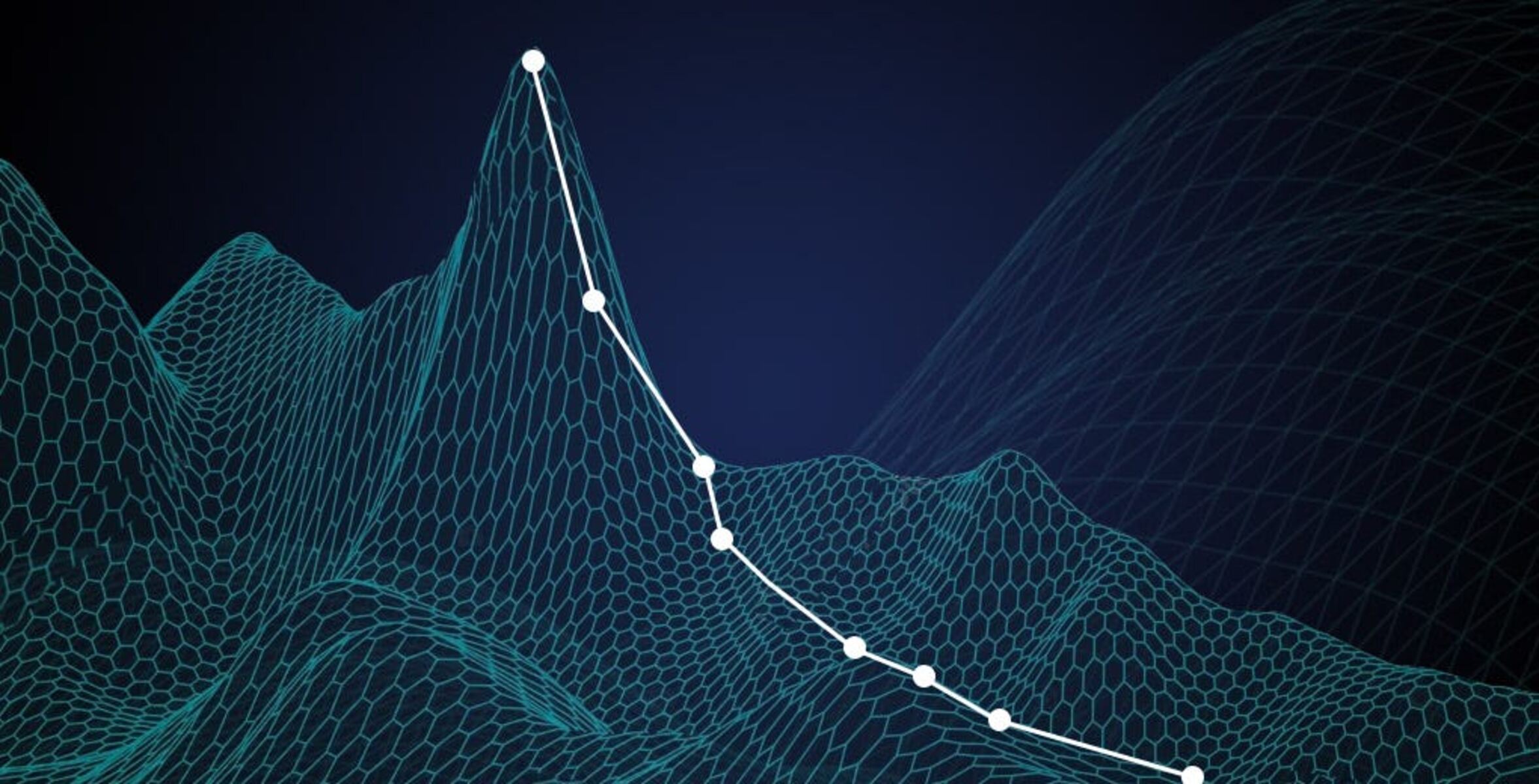
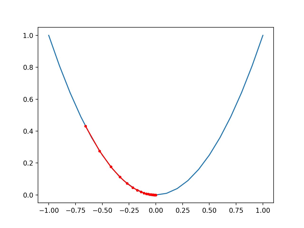
The main idea behind gradient descent is to follow the negative gradient direction of the loss function to gradually minimize it. The negative gradient points in the direction of steepest descent, indicating the direction in which the loss decreases the fastest. By taking steps in the negative gradient direction, the algorithm moves closer to the optimal parameters that result in minimal loss.
There are three main variants of gradient descent:
1. Batch Gradient Descent: In batch gradient descent, the algorithm computes the gradients for all training examples in the dataset and updates the parameters based on the average gradient over the entire dataset. This method ensures accurate estimation of the true gradient but can be computationally expensive for large datasets.
2. Stochastic Gradient Descent (SGD): Stochastic gradient descent updates the parameters after each individual training example. It randomly samples one data point at a time to compute the gradient. SGD is computationally efficient and can handle large datasets efficiently. However, due to the high variance introduced by using only one data point at a time, the optimization process can be more noisy and may require more iterations to converge.
3. Mini-Batch Gradient Descent: Mini-batch gradient descent is a compromise between batch gradient descent and stochastic gradient descent. It computes the gradients using a small random subset of training examples called mini-batches. This approach provides a balance between the computational efficiency of SGD and the stability of batch gradient descent, making it a commonly used variant in practice.
Irrespective of the variant used, the gradient descent algorithm typically involves the following steps:
1. Initialize the parameters: The algorithm starts by initializing the model parameters to some initial values.
2. Compute the loss: For each training example, the algorithm computes the difference between the predicted and actual values and calculates the loss function.
3. Calculate the gradients: The algorithm calculates the gradients of the loss function with respect to the parameters, indicating the direction and magnitude of the steepest descent that will reduce the loss.
4. Update the parameters: The parameters are updated by taking steps in the negative gradient direction, scaled by a learning rate. The learning rate determines the step size and influences the speed of convergence.
5. Repeat steps 2-4: The algorithm repeats steps 2-4 for a predetermined number of iterations or until a convergence criterion is met.
Gradient descent continues iterating through the dataset, updating the parameters until it finds a set of parameters that minimize the loss function to an acceptable level or until it reaches a predefined stopping criterion.
Gradient descent is a fundamental algorithm in machine learning and is widely used in various models, including linear regression, logistic regression, neural networks, and many more. Its simplicity and effectiveness make it a go-to optimization technique for improving model performance and achieving accurate predictions.
Backpropagation and Gradients
Backpropagation is a critical algorithm in training neural networks, and it heavily relies on the concept of gradients. It allows for efficient calculation of gradients throughout the layers of a neural network, enabling the network to learn and improve its performance.
The backpropagation algorithm works by propagating the error backward through the network, calculating the gradients of the loss function with respect to the parameters at each layer. These gradients provide insights into how the parameters should be adjusted to minimize the loss and improve the network’s predictions.
When a neural network processes a training example, it goes through a series of forward passes, where the inputs are transformed at each layer, finally producing an output. The difference between the predicted output and the true output is quantified using a loss function.
During the backward pass of backpropagation, the gradients of the loss function are calculated using the chain rule. The gradients are computed starting from the output layer and progressively propagated backward to previous layers, allowing for an efficient calculation of the gradients across the entire network.
At each layer, the gradients are used to update the parameters, such as the weights and biases, by taking steps in the negative gradient direction. These parameter updates enable the network to iteratively learn and adjust its parameters to minimize the loss function and improve its predictions.
The backpropagation algorithm effectively distributes the error across the layers of the network, giving each parameter responsibility for contributing to the overall error. It allows for the identification of weak connections or parameters that have a more significant impact on the loss, enabling focused optimization efforts.
It is crucial to mention that backpropagation combines the concept of gradients with gradient descent optimization. The gradients calculated during the backpropagation process are used to update the network’s parameters using techniques like stochastic gradient descent or mini-batch gradient descent.
Backpropagation has played a pivotal role in the success of deep learning, enabling the training of complex neural networks with numerous layers and millions of parameters. It has revolutionized the field of machine learning and has led to advancements in various areas, including computer vision, natural language processing, and reinforcement learning.
By efficiently calculating and utilizing gradients during the backpropagation process, neural networks can learn complex patterns and relationships in data, making them highly effective in solving a wide range of machine learning tasks.
Challenges and Limitations of Gradients in Machine Learning
While gradients are a powerful tool in machine learning, they are not without challenges and limitations. Understanding these limitations is crucial for practitioners to be aware of potential issues and develop strategies to address them. Let’s explore some of the key challenges and limitations associated with gradients in machine learning.
1. Vanishing and Exploding Gradients: In deep neural networks, the backpropagation algorithm can suffer from vanishing or exploding gradients. Vanishing gradients occur when the gradient values become extremely small as they propagate back through the layers, making it difficult for the network to learn effectively. Conversely, exploding gradients occur when the gradient values become extremely large, leading to unstable updates and slower convergence. To mitigate these issues, techniques like gradient clipping and initializing the network weights properly can be used.
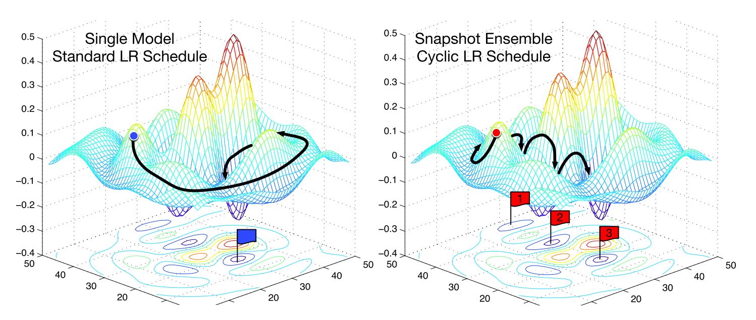
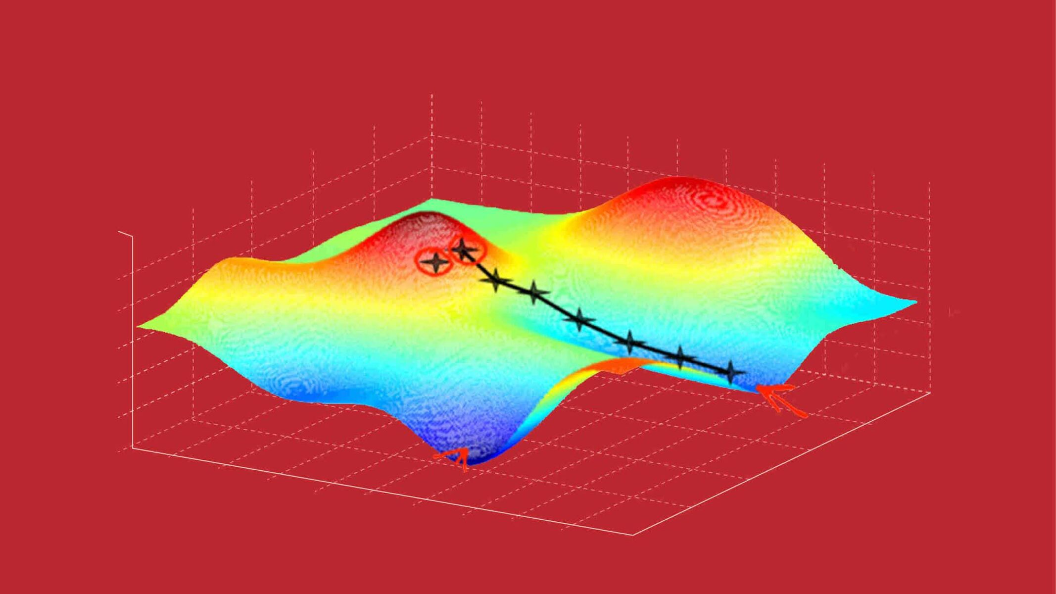
2. Local Optima and Plateaus: Gradients rely on the assumption that the loss function is smooth and convex, with a single global minimum. However, in complex optimization landscapes, there can be multiple local optima, making it challenging for gradient-based algorithms to find the global minimum. Additionally, plateaus, regions of the loss landscape with very flat gradients, can slow down optimization as the gradients provide little guidance. Techniques like adaptive learning rate schedules, momentum, and higher-order optimization methods can help overcome these challenges.
3. Computational Complexity: Calculating gradients can be computationally expensive, especially when dealing with large datasets or complex models. For deep neural networks with millions of parameters, the computational cost of computing gradients for all parameters at each iteration can be prohibitive. To address this, techniques like mini-batch gradient descent, parallel computing, and distributed training can be employed to reduce the computational burden.
4. Noisy or Inconsistent Gradients: In certain scenarios, the gradient estimates can be noisy or inconsistent, leading to unstable optimization. This can occur when using small mini-batches or in the presence of noisy or unbalanced data. Techniques like batch normalization, regularization, or data augmentation can help stabilize gradient estimates and improve optimization performance.
5. Non-differentiable or Discontinuous Functions: Gradients rely on the differentiability of the loss function and other components of the model. However, some functions employed in machine learning, such as max pooling or certain types of activation functions, are non-differentiable or discontinuous at certain points. These non-differentiable components can pose challenges in gradient-based optimization. Techniques like subgradients or relaxed optimization can be used in such cases.
6. Curse of Dimensionality: As the number of parameters or features in a model increases, the optimization problem becomes more complex. The search space for the optimal parameters becomes exponentially larger, making it harder for gradient-based algorithms to converge. Techniques like dimensionality reduction, regularization, or feature selection can help alleviate the curse of dimensionality and improve optimization.
Despite these challenges and limitations, gradients remain a fundamental tool in machine learning optimization. By understanding these limitations and employing appropriate techniques, practitioners can navigate around them and leverage gradients effectively to improve model performance and achieve accurate predictions.
Conclusion
Gradients are an integral part of machine learning, providing essential information about the direction and magnitude of the steepest ascent or descent of a function. They play a pivotal role in optimizing models and improving their performance by guiding algorithms to update parameters and minimize loss.
Throughout this article, we have explored the significance of gradients in machine learning. We learned that gradients allow algorithms to efficiently explore the parameter space, determine feature importance, and optimize models using techniques like gradient descent. We discussed different types of gradients, including batch gradient, stochastic gradient, mini-batch gradient, conditional gradient, natural gradient, and the use of the Hessian matrix.
Moreover, we examined the backpropagation algorithm, which relies on gradients to train neural networks effectively. We also showcased the challenges and limitations of gradients in machine learning, including vanishing and exploding gradients, local optima, computational complexity, noisy gradients, non-differentiable functions, and the curse of dimensionality.
Despite these challenges, gradients remain a crucial tool for optimizing models in machine learning. They enable algorithms to navigate complex parameter spaces, learn from data, and make accurate predictions. By understanding these challenges and employing appropriate strategies, practitioners can harness the power of gradients to improve model performance and unlock valuable insights.
In conclusion, gradients form the backbone of optimization algorithms in machine learning. They offer a powerful mechanism for learning from data and iteratively updating model parameters. As machine learning continues to advance, further research and innovation in gradient-based optimization techniques will undoubtedly contribute to the development of more efficient and accurate models.