What is an Optimizer in Machine Learning?
In the field of machine learning, an optimizer is a critical component used to adjust the parameters of a model in order to minimize the error or maximize the performance of a learning algorithm. It plays a crucial role in the training process by optimizing the weights and biases of the model based on the input data.
The goal of an optimizer is to find the optimal set of parameters that minimizes the loss function, which quantifies the error between the predicted values of the model and the actual values. By iteratively adjusting the parameters, the optimizer steers the model towards convergence, where the loss is minimized and the model starts making accurate predictions.
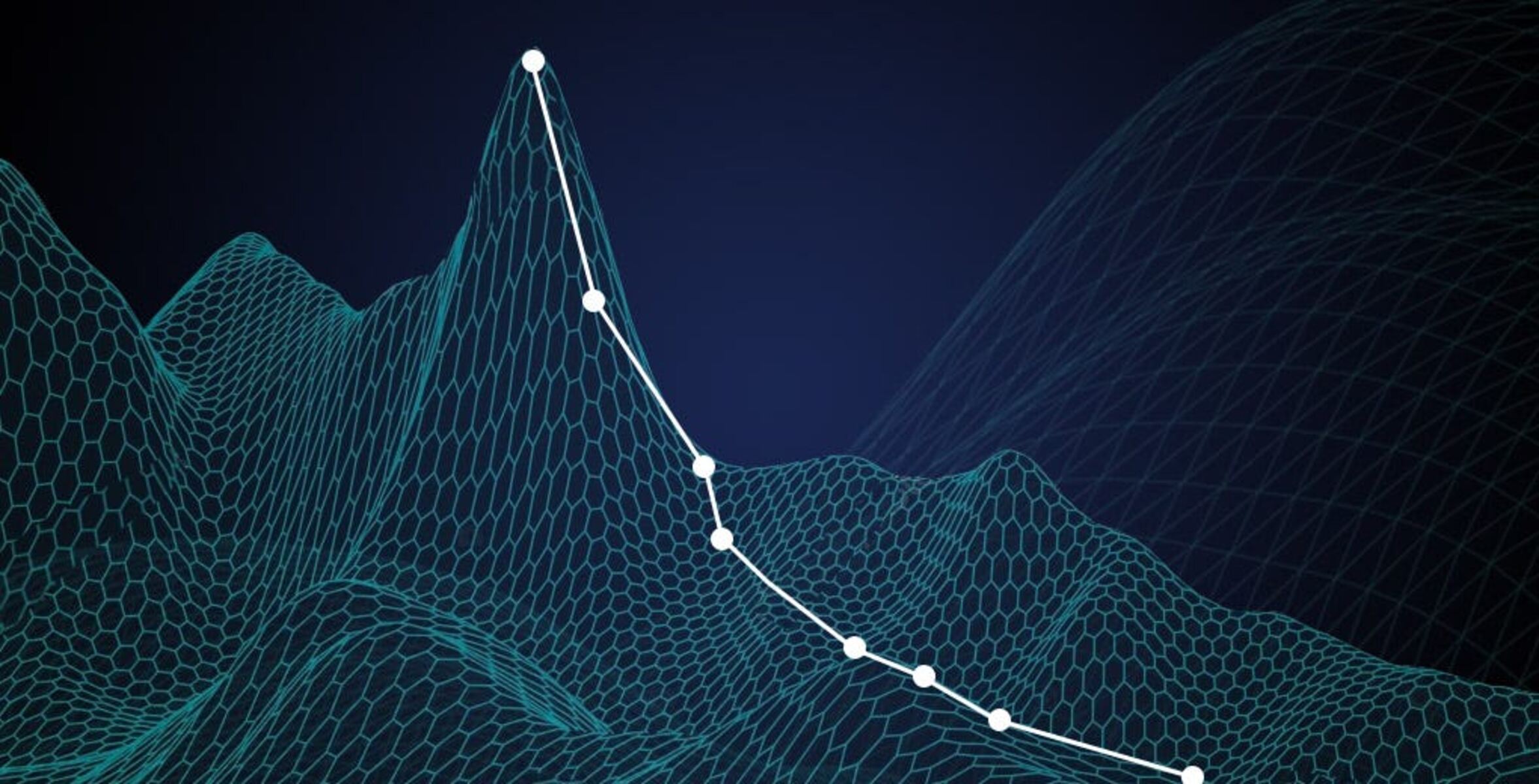
The optimization process can be seen as navigating a complex landscape with multiple peaks and valleys, where each peak denotes a different configuration of the model’s parameters. The optimizer’s job is to locate the global or local minimum, which represents the best configuration for the model.
There are various optimization algorithms available, each with its own strengths and weaknesses. These algorithms are designed to efficiently search the parameter space and converge to an optimal solution. Gradient-based optimizers, such as Gradient Descent and its variants, are commonly used in machine learning due to their simplicity and effectiveness.
Overall, an optimizer plays a crucial role in training machine learning models. It fine-tunes the model’s parameters by minimizing the error and improving the overall performance of the model. By utilizing various optimization algorithms, researchers and practitioners are able to tackle a wide range of machine learning problems and achieve state-of-the-art results.
How Does the Optimizer Work?
The optimizer in machine learning works by iteratively adjusting the parameters of a model to minimize the error or maximize the performance of the learning algorithm. It follows a predefined optimization algorithm to navigate the parameter space and find the optimal configuration for the model.
At the beginning of the training process, the model is initialized with random parameter values. The optimizer then evaluates the current performance of the model by calculating the loss function, which quantifies the error between the predicted values and the actual values.
Based on the calculated loss, the optimizer determines the direction and magnitude of the parameter updates. It makes small adjustments to the weights and biases of the model to minimize the loss over each iteration. This process is repeated until the model converges to an optimal solution, where the loss is minimized and the model achieves satisfactory performance.
The optimizer uses the concept of gradients, which are derivatives of the loss function with respect to the parameters. By calculating the gradients, the optimizer determines the slope of the loss function and updates the parameters accordingly. This is known as the gradient descent algorithm.
There are different variants of gradient-based optimizers, such as Stochastic Gradient Descent (SGD), Adam, RMSprop, and AdaGrad, which apply different strategies to adjust the parameters. SGD randomly selects a subset of training examples for each iteration, making it computationally efficient. Adam combines the advantages of both Adaptive Moment Estimation (Adam) and Root Mean Square Propagation (RMSprop) to improve convergence. RMSprop adapts the learning rate for each parameter based on the moving average of the squared gradients. AdaGrad adapts the learning rate based on the historical gradients for each parameter.
By efficiently updating the parameters using these optimization algorithms, the optimizer helps the model learn from the training data and generalize to unseen data. It plays a crucial role in the success of machine learning models by fine-tuning the parameters and optimizing the performance.
Popular Optimizers in Machine Learning
In the field of machine learning, there are several popular optimizers that are widely used to train models and optimize their performance. These optimizers vary in their approach and strategy to adjust the parameters of the model. Here are some of the most commonly used optimizers:
1. Gradient Descent
Gradient Descent is a widely used optimization algorithm that adjusts the parameters in the direction opposite to the gradient of the loss function. It starts with random initial values for the parameters and updates them iteratively based on the calculated gradients. Gradient Descent can be further classified into different variants, such as Batch Gradient Descent, Mini-Batch Gradient Descent, and Stochastic Gradient Descent (SGD).
2. Stochastic Gradient Descent (SGD)
Stochastic Gradient Descent (SGD) is a variant of Gradient Descent that randomly selects a subset of training examples (batch) for each iteration. It updates the parameters based on the gradients calculated from this subset. SGD is computationally efficient and often converges faster than traditional Gradient Descent.
3. Adam
Adam, short for Adaptive Moment Estimation, is an adaptive learning rate optimization algorithm that combines the strategies of both RMSprop and Momentum. It adapts the learning rate for each parameter based on the first-order moments (the mean) and the second-order moments (the uncentered variance) of the gradients. Adam is known for its good convergence properties and robustness to noisy or sparse gradients.
4. RMSprop
Root Mean Square Propagation (RMSprop) is an optimization algorithm that adapts the learning rate for each parameter based on the moving average of the squared gradients. It divides the learning rate by a running average of the history of squared gradients to speed up convergence. RMSprop is especially effective in dealing with sparse data or non-stationary objectives.
5. AdaGrad
AdaGrad, short for Adaptive Gradient, is an optimization algorithm that adapts the learning rate for each parameter based on the historical gradients. It assigns a different learning rate to each parameter, with the learning rate decreasing for frequently occurring parameters. AdaGrad is effective in handling sparse data and is often used in natural language processing tasks.
These are just a few examples of popular optimizers in machine learning. Depending on the nature of the problem and the properties of the data, different optimizers may yield different results. It is crucial to experiment with different optimizers to find the one that works best for a given task.
Gradient Descent
Gradient Descent is a widely used optimization algorithm in machine learning that is used to update the parameters of a model iteratively. It aims to minimize the loss function by adjusting the parameters in the direction opposite to the gradient of the loss function.
The basic idea behind Gradient Descent is to start with random initial values for the parameters and calculate the gradients of the loss function with respect to each parameter. The gradients indicate the slope of the loss function at a specific point, and moving in the opposite direction of the gradient allows us to descend the loss function and find the minimum.
There are different variants of Gradient Descent, each with its own approach to updating the parameters:
Batch Gradient Descent
Batch Gradient Descent computes the gradients using the entire training dataset. It calculates the gradients by summing up the gradients of each training example and then performs a parameter update. Although Batch Gradient Descent guarantees convergence to the global minimum, it can be computationally expensive for large datasets.
Mini-Batch Gradient Descent
Mini-Batch Gradient Descent is a compromise between Batch Gradient Descent and Stochastic Gradient Descent. It randomly selects a subset or mini-batch of training examples for each iteration and computes the gradients based on this mini-batch. This approach reduces the computational burden and still provides good convergence.
Stochastic Gradient Descent (SGD)
Stochastic Gradient Descent (SGD) takes the concept of Mini-Batch Gradient Descent further by selecting only one random training example for each iteration. SGD computes the gradients based on this single example and updates the parameters immediately. This approach is computationally efficient, but the parameter updates can be noisy, leading to fluctuations in the loss function.
The choice between these variants depends on the size of the dataset and the computational resources available. Batch Gradient Descent is suitable for smaller datasets, while Mini-Batch Gradient Descent and SGD are preferred for larger datasets.
Gradient Descent is a fundamental optimizer in machine learning, and its variants form the backbone of many optimization algorithms. By iteratively adjusting the parameters based on the gradients, Gradient Descent helps the model converge to an optimal set of parameter values and improve its performance.
Stochastic Gradient Descent (SGD)
Stochastic Gradient Descent (SGD) is a popular optimization algorithm used in machine learning for training models. It is a variant of Gradient Descent that updates the model’s parameters using a randomly selected subset of training examples for each iteration.
The main advantage of SGD over traditional Gradient Descent is its computational efficiency. Rather than evaluating the entire training dataset in each iteration, SGD only considers a small subset of examples, often referred to as a mini-batch. This makes it particularly useful for large datasets that do not fit into memory.
At each iteration, SGD randomly selects a mini-batch of training examples and computes the loss and gradients based on this subset. It then updates the model’s parameters using the gradients calculated from the mini-batch. By repeatedly performing these updates, SGD steers the model towards a minimum of the loss function.
One important characteristic of SGD is its stochastic nature. Due to the randomness in selecting mini-batches, the parameter updates in SGD can be noisy and result in fluctuations in the loss function. However, this stochastic nature can also help SGD escape local minima and explore different regions of the parameter space, leading to better generalization.
Despite its noise and fluctuations, SGD has proven to be a powerful optimization algorithm. It is widely used in deep learning as it enables training large neural networks efficiently. Additionally, the noise introduced by SGD can act as a form of regularization, preventing overfitting and improving the model’s ability to generalize to unseen data.
There are variations of SGD that further modify the basic algorithm. One such variation is mini-batch SGD, where the algorithm considers a batch of more than one but fewer than all training examples. This strikes a balance between the computational efficiency of SGD and the stability of traditional Gradient Descent.
In summary, Stochastic Gradient Descent is a popular optimization algorithm that updates the model’s parameters using randomly selected subsets of training examples. It offers computational efficiency, regularization through noise, and the ability to escape local optima. These qualities make SGD a valuable tool for training machine learning models, especially in large-scale and deep learning scenarios.
Adam
Adam, short for Adaptive Moment Estimation, is an optimization algorithm commonly used in machine learning. It combines the advantages of two other optimization methods, Adaptive Gradient Algorithm (AdaGrad) and Root Mean Square Propagation (RMSprop), to provide an efficient and effective approach for updating the parameters of a model.
The Adam optimizer adapts the learning rate for each parameter based on the first-order moments (the mean) and the second-order moments (the uncentered variance) of the gradients. It calculates exponentially decaying averages of past gradients and their square values, effectively estimating the first moment (mean) and the second moment (variance) of the gradients.
The algorithm uses this estimation of the mean and variance to update the parameters. It combines the benefits of AdaGrad, which scales the learning rate based on the historical gradients, and RMSprop, which adjusts the learning rate adaptively based on the moving average of the squared gradients.
The key advantage of Adam is its ability to handle sparse gradients and non-stationary objectives. By maintaining separate learning rates for each parameter, it can adaptively update the parameters based on their relevance to the optimization process. This makes Adam particularly effective in scenarios where different parameters may have different update requirements.
Additionally, Adam helps to overcome some of the limitations of other optimization algorithms. It exhibits good convergence properties and is robust to noisy or sparse gradients. The adaptive learning rate adjustment allows Adam to converge quickly and achieve good performance on a wide range of machine learning tasks.
Another important feature of Adam is the bias correction step. Since Adam calculates the first and second moments of the gradients using exponential moving averages, the estimates are biased towards zero, especially in the early stages of training. To correct this bias, Adam applies a correction factor to the bias-corrected estimates. This helps to improve the accuracy of the moment estimates and further enhances the performance of the optimizer.
In summary, Adam is an adaptive optimization algorithm that combines the benefits of AdaGrad and RMSprop. By adapting the learning rate based on the first and second moments of the gradients, Adam effectively updates the parameters and achieves good convergence. It is widely used in deep learning and other machine learning tasks due to its efficiency, robustness, and ability to handle non-stationary objectives.
RMSprop
RMSprop, short for Root Mean Square Propagation, is an optimization algorithm commonly used in machine learning. It is designed to address some of the limitations of traditional gradient-based optimization methods by adapting the learning rate for each parameter based on the historical gradients.
The main objective of RMSprop is to speed up convergence by adjusting the learning rate based on the moving average of the squared gradients. It divides the learning rate by the square root of the exponentially decaying average of the squared gradients. This normalization prevents the learning rate from getting too large when the gradients are consistently large, and vice versa when the gradients are consistently small.
The intuition behind RMSprop is that it adapts the learning rate differently for each parameter based on their recent gradient history. Gradients with larger magnitude will result in smaller learning rates, while gradients with smaller magnitude will result in larger learning rates. This adaptive adjustment of the learning rate helps to improve convergence and alleviate the problem of oscillations or divergences that can occur with a fixed learning rate.
Additionally, RMSprop is effective in dealing with sparse data or non-stationary objectives. By maintaining a moving average of the squared gradients, it adapts the learning rate according to the characteristics of the gradients encountered during training. This makes RMSprop particularly useful in scenarios where the gradients vary significantly across different parameters or data points.
One important feature of RMSprop is its ability to handle different learning rates for different parameters. It allows the algorithm to adjust the learning rate individually for each parameter, which can be beneficial when certain parameters require slower or faster updates compared to others.
Overall, RMSprop is a powerful optimization algorithm that adapts the learning rate based on the historical gradients. It provides an efficient and effective approach for training machine learning models. By normalizing the learning rate based on the moving average of the squared gradients, RMSprop allows for better convergence, improved stability, and enhanced performance in various machine learning tasks.
AdaGrad
AdaGrad, short for Adaptive Gradient, is an optimization algorithm commonly used in machine learning. It is designed to adaptively adjust the learning rate for each parameter based on the historical gradients, making it particularly useful for sparse data or non-stationary objective functions.
The main idea behind AdaGrad is to assign a different learning rate to each parameter based on the historical magnitudes of the gradients. It starts by accumulating the sum of the squared gradients for each parameter over time. This accumulation acts as a measure of how frequently a parameter has been updated, giving more weight to infrequently updated parameters and less weight to frequently updated parameters.
AdaGrad achieves this adjustment by dividing the learning rate by the square root of the accumulated sum of squared gradients. Parameters with larger gradients will have a smaller learning rate, while parameters with smaller gradients will have a larger learning rate. This approach allows AdaGrad to adaptively change the learning rate for each parameter, addressing the issue of vanishing or exploding gradients.
One key advantage of AdaGrad is its ability to handle sparse data. In many machine learning tasks, the input data is sparse, meaning that only a small portion of the features or inputs have non-zero values. Traditional optimization algorithms that treat all dimensions equally may assign excessive updates to the non-zero dimensions, leading to poor performance. AdaGrad mitigates this issue by scaling the learning rate inversely proportional to the square root of the accumulated sum of squared gradients, giving more emphasis to rarely occurring features or inputs.
However, one potential drawback of AdaGrad is that the learning rate tends to become overly small as the accumulation of squared gradients continues. This can hinder learning in later stages of training. To address this, other optimization algorithms such as RMSprop and Adam have been developed, which use different strategies to adapt the learning rate.
In summary, AdaGrad is an optimization algorithm that adjusts the learning rate for each parameter based on the historical gradients. It offers an adaptive approach for handling sparse data and non-stationary objective functions. While it has its limitations, AdaGrad serves as a key milestone in the development of optimization algorithms and has paved the way for further advancements in this field.
Choosing the Right Optimizer
Choosing the right optimizer is a critical decision in machine learning as it can significantly impact the training process and the performance of the model. Different optimizers have their strengths and weaknesses and may be more suitable for specific tasks or datasets. Here are some key factors to consider when selecting an optimizer:
1. Dataset and Problem
The characteristics of your dataset and problem play a significant role in determining the most appropriate optimizer. Consider the size of the dataset, the complexity of the data, and the nature of the problem you are trying to solve. For smaller datasets, traditional gradient-based optimizers like Gradient Descent or its variants may work well. For larger datasets, stochastic optimization algorithms like Stochastic Gradient Descent (SGD) or adaptive optimizers like Adam or RMSprop may be more efficient.
2. Model Architecture
The structure and complexity of your model can influence the optimizer choice. Deep neural networks with many layers and parameters often benefit from adaptive optimizers like Adam or RMSprop. These optimizers can help navigate the parameter space more effectively and speed up convergence. For simpler models, simpler optimizers like Gradient Descent or SGD may suffice.
3. Convergence Speed
If you have limited time or computational resources, the convergence speed of the optimizer becomes important. Adaptive optimizers like Adam and RMSprop are often faster in converging compared to traditional methods like Gradient Descent or SGD. However, it’s worth noting that faster convergence does not always guarantee better performance, so it’s important to strike a balance between speed and accuracy.
4. Noise Tolerance
Some optimizers, like SGD, introduce noise to the optimization process due to their stochastic nature. This noise can act as a regularizer, preventing overfitting and improving generalization. If you have a complex model or a limited amount of training data, using an optimizer that introduces noise, like SGD, could be beneficial.
5. Experimentation
Ultimately, the choice of optimizer may require experimentation and empirical evaluation. It is common practice to try out different optimizers and compare their performance on a validation set. This allows you to assess which optimizer works best for your specific problem and dataset.
Remember that the choice of optimizer is not fixed and can be reevaluated and changed during the training process. Different optimizers may have different effects at different stages of training, so it’s important to monitor the performance and make adjustments if necessary.
By considering these factors and evaluating the trade-offs, you can make an informed decision about the optimizer that is most suitable for your machine learning task.
Optimization Techniques: Beyond Traditional Optimizers
While traditional optimizers like Gradient Descent, Stochastic Gradient Descent (SGD), Adam, RMSprop, and AdaGrad are widely used in machine learning, there are several optimization techniques that go beyond these traditional approaches. These techniques aim to further improve the performance, convergence speed, and robustness of machine learning models. Here are a few notable optimization techniques:
1. Momentum Optimization
Momentum optimization introduces the concept of momentum to the parameter updates. It accumulates a velocity vector that determines the direction and speed of movement through the parameter space. This technique helps the optimization process by accelerating convergence and reducing oscillations, especially in areas with high curvatures or noisy gradients.
2. Nesterov Accelerated Gradient (NAG)
Nesterov Accelerated Gradient (NAG) is an optimization technique that enhances momentum optimization. It adjusts the parameter updates by taking into account the momentum in the step-ahead position. By considering the momentum, NAG improves the convergence speed and allows for more accurate updates in comparison to traditional momentum optimization.
3. Adadelta
Adadelta is an adaptive learning rate optimization technique that aims to overcome the limitations of AdaGrad. Unlike AdaGrad, Adadelta accumulates a running average of the gradients and the updates. It further normalizes the learning rates by dividing the parameter updates by the exponentially decaying average of the squared updates. Adadelta helps avoid the diminishing learning rate problem faced by AdaGrad, improving stability and convergence.
4. RMSprop with Nestrov Momentum (RMSprop with NAG)
This technique is a combination of RMSprop and Nesterov Accelerated Gradient (NAG). It incorporates the adaptive learning rate of RMSprop and the momentum concept of NAG. By utilizing both of these techniques, RMSprop with NAG achieves better optimization performance, faster convergence, and improved stability in comparison to using either technique alone.
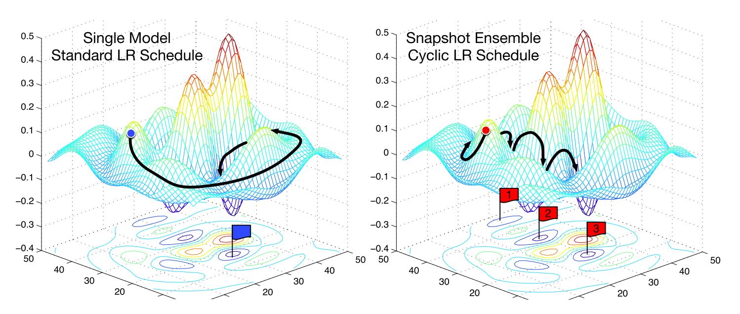
5. Cyclical Learning Rates
Cyclical Learning Rates (CLR) is a learning rate policy that dynamically adjusts the learning rate within a specified range during training. Instead of using a fixed learning rate, CLR explores a range of learning rates, periodically increasing and decreasing the learning rate at set intervals. This cyclic exploration helps the model escape from local minima and saddle points, leading to improved optimization and potential better generalization.
These optimization techniques, along with many others, are continuously being developed and researched to improve the training process of machine learning models. Depending on the problem, model architecture, and dataset, incorporating these advanced techniques can provide additional benefits and further enhance the performance of your models.
Conclusion
Optimizers are essential components in machine learning that play a crucial role in training models and improving their performance. Choosing the right optimizer can greatly impact the convergence speed, stability, and generalization of the model. By understanding the different optimization algorithms and their characteristics, you can make informed decisions to optimize your machine learning models.
In this article, we explored the concept of optimizers and their role in machine learning. We discussed popular optimizers such as Gradient Descent, Stochastic Gradient Descent (SGD), Adam, RMSprop, and AdaGrad, along with their strengths and applications. We also delved into considerations for choosing the right optimizer, such as dataset characteristics, model architecture, convergence speed, noise tolerance, and the importance of experimentation.
Furthermore, we explored optimization techniques beyond traditional optimizers, including Momentum Optimization, Nesterov Accelerated Gradient (NAG), Adadelta, RMSprop with NAG, and Cyclical Learning Rates (CLR). These advanced techniques offer additional means to enhance the training process and improve the performance of machine learning models.
It’s worth noting that the choice of optimizer is not a one-size-fits-all approach. Depending on the specific problem, dataset, and model, different optimizers may yield varying results. It is important to experiment with different optimizers, monitor their performance, and refine the choice based on empirical observations.
In conclusion, optimizers are powerful tools that greatly impact the performance of machine learning models. By understanding the strengths and characteristics of different optimizers, and considering the specific requirements of your task, you can choose the right optimizer and optimize your models for better performance and convergence.