What Is A Linear Model In Machine Learning

Introduction

Welcome to the fascinating world of machine learning! In this digital era, where vast amounts of data are generated every second, machine learning models play a crucial role in extracting valuable insights and making predictions. One such model is the linear model, which forms the foundation of many machine learning algorithms.

Linear models are mathematical equations that establish a linear relationship between input variables, also known as features, and the output variable. They have been widely used in various fields, including finance, healthcare, marketing, and more. Understanding the basics of linear models is essential for anyone venturing into the field of machine learning.

In this article, we will shed light on what exactly a linear model is, how it works, its types, advantages, limitations, and key concepts related to linear modeling. We will also explore real-world applications and the steps involved in building and evaluating a linear model. By the end of this article, you will have a solid understanding of linear models and their significance in the realm of machine learning.

So, whether you are an aspiring data scientist, a seasoned machine learning enthusiast, or simply curious about how algorithms can unravel patterns in data, join us on this exciting journey into the world of linear models!

Definition of Linear Model

A linear model, also known as a linear regression model, is a mathematical representation of the relationship between one or more input variables and an output variable, where the relationship is assumed to be linear. It assumes that there is a linear relationship between the input variables and the output variable, meaning that the change in the input variables results in a proportional change in the output variable.

In terms of equation, a linear model can be represented as:

y = β₀ + β₁x₁ + β₂x₂ + … + βₙxₙ + ε

where:

y is the output variable that we are trying to predict
β₀, β₁, β₂, …, βₙ are the coefficients or weights of the input variables
x₁, x₂, …, xₙ are the input variables
ε is the error term, which represents the deviation between the predicted and actual values of the output variable

The goal of a linear model is to estimate the values of the coefficients β₀, β₁, β₂, …, βₙ that minimize the overall error between the predicted and actual values of the output variable. This is typically achieved using a technique called ordinary least squares (OLS) regression.

Linear models are widely used due to their simplicity, interpretability, and effectiveness in many scenarios. They form the basis for more complex machine learning algorithms such as logistic regression, support vector machines, and neural networks.

It is important to note that linear models make certain assumptions, including linearity, independence of error terms, constant variance of error terms, and absence of multicollinearity. Violation of these assumptions can affect the accuracy and reliability of the model’s predictions.

Now that we have a clear understanding of what a linear model is, let’s delve deeper into how it works and the various types of linear models.

How Does a Linear Model Work?

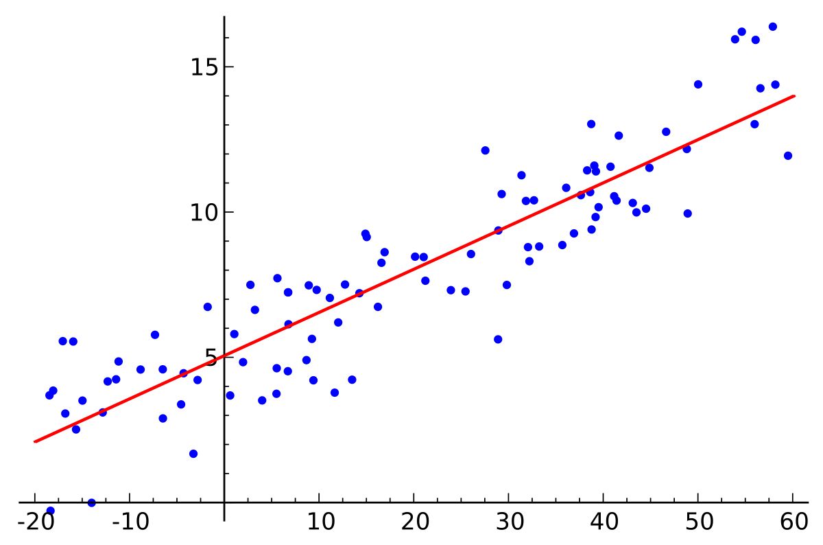
Linear models work by fitting a line or a hyperplane to the data points in order to predict the value of the output variable based on the input variables. The process involves estimating the values of the coefficients that best represent the relationship between the input and output variables.

To understand how a linear model works, let’s consider a simple example. Suppose we have a dataset with two input variables, x₁ and x₂, and we want to predict the output variable, y. The linear model equation in this case would be:

y = β₀ + β₁x₁ + β₂x₂ + ε

The goal of the model is to estimate the values of β₀, β₁, and β₂ that minimize the error between the predicted values and the actual values of y. The process of estimating these coefficients involves the use of mathematical techniques such as least squares regression.

During the training phase, the linear model analyzes the relationship between the input variables and the output variable by minimizing the sum of the squared differences between the predicted and actual values. This optimization process adjusts the coefficients iteratively until the model reaches the best possible fit to the data.

Once the coefficients are estimated, the linear model can be used to make predictions on new, unseen data. By plugging in the values of the input variables into the equation, the model calculates the corresponding predicted value of the output variable.

It’s worth noting that linear models work well when the relationship between the input and output variables is roughly linear. If the relationship is non-linear, the model may not accurately capture the patterns in the data. In such cases, non-linear models or feature engineering techniques may be more suitable.

Furthermore, linear models can handle both continuous and categorical input variables by properly encoding the categorical variables using techniques like one-hot encoding.

In the next section, we will explore different types of linear models that are commonly used in machine learning.

Types of Linear Models

Linear models come in various forms, each designed to handle different scenarios and data types. Let’s explore some of the commonly used types of linear models:

Simple Linear Regression: This is the most basic form of linear regression, where there is only one input variable. The relationship between the input variable and the output variable is represented by a straight line, and the model estimates the slope and intercept of that line.
Multiple Linear Regression: In multiple linear regression, there are multiple input variables. The model estimates the coefficients for each input variable to determine their respective impact on the output variable. The relationship is represented by a hyperplane in a higher-dimensional space.
Ridge Regression: Ridge regression is a variant of linear regression that introduces a regularization term to the cost function. This helps prevent overfitting of the model by imposing a penalty on large coefficient values. Ridge regression is particularly useful when dealing with multicollinearity, where input variables are highly correlated.
Lasso Regression: Similar to ridge regression, lasso regression also adds a regularization term to the cost function. However, lasso regression uses the L1 norm instead of the L2 norm, which encourages sparse coefficient values by driving some coefficients to zero. This makes lasso regression valuable in feature selection, as it automatically selects the most relevant features for the model.
ElasticNet Regression: ElasticNet regression combines the properties of ridge regression and lasso regression by using a combination of the L1 and L2 norms in the regularization term. This allows for both coefficient shrinkage and automatic feature selection.
Logistic Regression: Contrary to its name, logistic regression is a linear model used for binary classification. It estimates the probability of the output variable belonging to a particular class based on the input variables. Logistic regression is widely used in machine learning, particularly in problems where the outcome is categorical.

These are just a few examples of linear models. Other variations and extensions, such as polynomial regression, stepwise regression, and generalized linear models, exist to handle different types of relationships and data distributions.

Now that we have explored the types of linear models, let’s move on to discussing the advantages and limitations of using linear models in machine learning.

Advantages of Linear Models

Linear models offer several advantages that make them widely used in machine learning applications. Let’s take a closer look at some of the key advantages:

Simplicity: Linear models are straightforward and easy to understand, making them accessible even to those new to machine learning. The linear relationship assumption allows for intuitive interpretations of coefficients, providing insight into the effects of input variables on the output variable.
Interpretability: Due to their simplicity, linear models provide interpretability, allowing us to understand the impact of each input variable on the output variable. Coefficients can be directly interpreted as the change in the output variable for a one-unit change in the corresponding input variable, holding other variables constant.
Efficiency: Linear models are computationally efficient and can handle large datasets with relatively low computational resources. This makes them suitable for real-time and online learning scenarios.
Robustness to Outliers: Linear models are robust to the presence of outliers in the dataset. Outliers have less impact on the overall model’s fit due to the use of techniques such as least squares regression.
Feature Selection: With the use of techniques such as ridge regression and lasso regression, linear models can automatically select the most relevant features for prediction. This simplifies the model and reduces the risk of overfitting.
Foundation for Complex Models: Linear models serve as the building blocks for more complex machine learning algorithms. Many advanced algorithms, such as support vector machines and neural networks, are based on the concepts and principles of linear models.

Although linear models offer many advantages, it is important to acknowledge their limitations and understand when they may not be the most suitable choice. In the next section, we will discuss the limitations of linear models in machine learning.

Limitations of Linear Models

Despite their usefulness, linear models have certain limitations that restrict their applicability in certain scenarios. Here are some notable limitations:

Assumption of Linearity: Linear models assume a linear relationship between the input variables and the output variable. If the true relationship is nonlinear, the model may not capture the underlying patterns effectively.
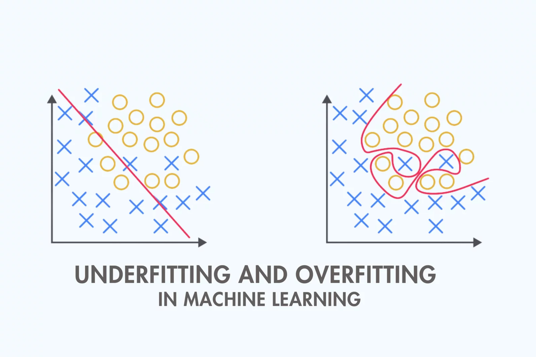
Limited Complexity: Linear models have a limited capacity to represent complex relationships, especially if interactions or nonlinearity are prominent in the data. This can result in underfitting, where the model fails to capture the true underlying patterns due to its simplicity.
Multicollinearity: Multicollinearity occurs when input variables are highly correlated with each other. This can pose challenges in estimating the coefficients accurately, as it becomes difficult to determine the independent effect of each variable on the output.
Outliers: While linear models are generally robust to outliers, extreme outliers can still have a significant impact on the model’s fit. Outliers that do not follow the linear relationship assumption can distort the model’s predictions.
Limited Feature Engineering: Linear models rely on the input variables being appropriately transformed and represented. If the relationship between the input and output variables is nonlinear, additional feature engineering techniques, such as polynomial features or interactions, may be required to improve the model’s accuracy.
Overfitting: Linear models can also suffer from overfitting if the model becomes too complex or the number of input variables exceeds the number of data points. Overfitting occurs when the model fits the training data too closely, resulting in poor performance on unseen data.
Binary Classification Limitation: Logistic regression, a type of linear model used for binary classification, assumes a linear relationship between the input variables and the log-odds of the probability. This assumption may not hold if the relationship is highly nonlinear, leading to inaccurate predictions.

While linear models have their limitations, they remain valuable tools in many machine learning applications. It is important to consider the specific characteristics of the dataset and the problem at hand to determine if a linear model is appropriate or if a more complex model should be explored.

Now that we understand the limitations, let’s move on to discussing some key concepts involved in linear modeling.

Key Concepts in Linear Modeling

Linear modeling involves several key concepts that are important to grasp in order to build and interpret linear models effectively. Let’s explore some of these key concepts:

Coefficients: Coefficients, also known as weights, represent the slopes of the input variables in a linear model. They quantify the impact of each input variable on the output variable. Positive coefficients indicate a positive relationship, while negative coefficients indicate a negative relationship.
Intercept: The intercept, or the bias term (β₀), represents the baseline value of the output variable when all input variables are zero. It determines the starting point of the line or hyperplane in the linear model.
R-squared: R-squared measures the proportion of the variance in the output variable that is explained by the linear model. It ranges from 0 to 1, with a higher value indicating a better fit of the model to the data.
P-value: P-value is a measure of the statistical significance of a coefficient. It indicates the probability of observing a coefficient as extreme as the estimated one, assuming the null hypothesis is true (i.e., no relationship between the input and output variables). A low p-value suggests a significant relationship.
Residuals: Residuals are the differences between the predicted and actual values of the output variable. In linear modeling, minimizing the sum of squared residuals is the objective, as it represents the error of the model. Residual analysis helps assess the model’s goodness of fit and identify potential outliers or violations of assumptions.
Variance Inflation Factor (VIF): VIF is a measure of multicollinearity, indicating the extent to which the variance of a coefficient is increased due to its correlation with other input variables. It helps identify highly correlated variables that may affect coefficient estimation and interpretation.
Cross-validation: Cross-validation is a technique used to assess a model’s performance by evaluating its ability to generalize to unseen data. It involves splitting the data into training and testing sets, fitting the model on the training set, and evaluating its performance on the testing set. This helps estimate how well the model will perform on new, unseen data.

Understanding these key concepts is crucial for interpreting the results of a linear model, making informed decisions about feature selection, assessing model performance, and identifying potential issues or violations of assumptions.

With a grasp of these concepts, let’s now explore the applications of linear models in various machine learning scenarios.

Applications of Linear Models in Machine Learning

Linear models find wide-ranging applications in the field of machine learning. Let’s explore some of the common areas where linear models are utilized:

Regression Analysis: Linear regression models are extensively used for regression analysis, where the goal is to predict a continuous output variable. Industries such as finance, economics, and social sciences leverage linear regression to forecast stock prices, estimate housing prices, analyze the impact of advertising on sales, and investigate the relationship between variables.
Classification: Despite their name, linear models like logistic regression are highly effective for binary classification tasks. They are employed in various domains, including healthcare (diagnostic prediction), fraud detection, spam filtering, sentiment analysis, and credit risk assessment. Linear models provide interpretable outputs in these cases, allowing decision-makers to understand the factors influencing classification outcomes.
Feature Selection: The ability of linear models to estimate the importance of input variables makes them valuable for feature selection. By examining the coefficients, researchers and data scientists can identify the most influential features for prediction or gain insights into the underlying process being modeled.
Anomaly Detection: Linear models can aid in detecting anomalies in datasets. By building a model with normal data points, any instances that deviate significantly from the predicted values can be flagged as anomalies. This approach is commonly used in fraud detection, network intrusion detection, and outlier identification in various domains.
Dimensionality Reduction: Principal Component Analysis (PCA), a linear dimensionality reduction technique, utilizes linear models to transform high-dimensional data into lower-dimensional representations. It identifies the directions in which the data exhibits the most variation and reduces the dimensionality while retaining the most important information. PCA finds applications in image processing, genetics, and text analysis.
Time Series Analysis: Linear models form the basis of time series analysis methods like AutoRegressive Integrated Moving Average (ARIMA) and Exponential Smoothing models. By capturing the linear dependencies among past observations, linear models assist in forecasting future values of a time series variable. They are commonly used in forecasting stock prices, weather data analysis, and demand forecasting.

The versatility of linear models ensures their utility across various industries and machine learning tasks. However, it is crucial to determine if the assumptions of linearity and other necessary conditions are met before applying them to a specific problem.

Now that we understand the applications, let’s proceed to discussing the steps involved in building a linear model.

Steps to Build a Linear Model

Building a linear model involves several steps, from data preparation to model evaluation. Let’s explore the key steps involved in building a linear model:

Data Collection and Preprocessing: The first step is to gather the relevant data for your problem. This may involve data collection from various sources, cleaning the data by handling missing values and outliers, and performing necessary transformations such as scaling or normalization.
Feature Selection and Engineering: Identify the input variables, or features, that are most relevant to your problem. Consider removing irrelevant or redundant features through techniques like correlation analysis or stepwise regression. Additionally, you may need to engineer new features by transforming or combining existing ones to improve the model’s performance.
Train-Test Split: Split your dataset into a training set and a testing set. The training set will be used to train the model, while the testing set will be used to evaluate its performance on unseen data. Typically, a ratio of 70:30 or 80:20 is used for the train-test split.
Model Training: Fit the linear model to the training data using estimation techniques such as ordinary least squares regression. This involves finding the optimal values for the coefficients that minimize the error between the predicted and actual values of the output variable.
Model Evaluation: Evaluate the performance of the trained model using appropriate evaluation metrics. For regression tasks, common metrics include mean squared error (MSE) and R-squared. For classification tasks, metrics like accuracy, precision, recall, and F1 score are used to assess the model’s performance.
Model Tuning and Improvement: If the model’s performance is not satisfactory, consider tuning the model by adjusting hyperparameters, trying different regularization techniques, or selecting different features. Iteratively refine the model to achieve the desired performance.
Model Interpretation: Interpret the learned coefficients to understand the relationship between the input variables and the output variable. Higher magnitude coefficients indicate stronger effects on the output variable, while the sign of the coefficient (positive or negative) indicates the direction of the relationship.
Prediction: Once the model is trained and evaluated, it can be used to make predictions on new, unseen data. Simply plug in the values of the input variables into the model equation to obtain the predicted value of the output variable.

These steps form a general framework for building a linear model. It’s important to note that the specific implementation may vary depending on the tools, algorithms, and programming languages used. Remember to consider the assumptions, limitations, and requirements of linear regression during each step of the process.

Now that we have covered the steps involved in building a linear model, let’s move on to discussing how to evaluate and improve the performance of a linear model.

Evaluating and Improving a Linear Model

Evaluating and improving the performance of a linear model is a crucial step in the machine learning workflow. Let’s explore the key aspects of evaluating and improving a linear model:

Evaluation Metrics: Choose appropriate evaluation metrics to assess the model’s performance. For regression tasks, metrics such as mean squared error (MSE), root mean squared error (RMSE), and R-squared can measure the goodness of fit. For classification tasks, metrics like accuracy, precision, recall, and F1 score provide insights into the model’s predictive ability.
Cross-Validation: Perform cross-validation to evaluate the model’s performance on various subsets of the data. Techniques like k-fold cross-validation can estimate the model’s generalization ability and help assess its stability and robustness.
Residual Analysis: Analyze the residuals to assess the model’s assumptions and identify any patterns or outliers. Plotting the residuals against predicted values can help identify heteroscedasticity (unequal variance) or nonlinearity in the relationship between the input and output variables.
Regularization: Consider using regularization techniques like ridge regression or lasso regression to reduce overfitting and improve the model’s generalization ability. These techniques introduce a penalty term to the cost function, encouraging simpler models and adjusting the coefficients accordingly.
Feature Engineering: Continuously explore and engineer new features that might enhance the model’s performance. This could involve transforming variables, creating interaction terms, or incorporating domain knowledge to capture more complex relationships between the input and output variables.
Feature Scaling: Scale or normalize the input variables to ensure they are on a similar scale. This helps prevent variables with larger magnitudes from dominating the model’s estimation process. Common techniques include standardization (subtracting the mean and dividing by the standard deviation) or normalization (scaling values between 0 and 1).
Outlier Treatment: Identify and handle outliers that may significantly impact the model’s performance. Removing or transforming outliers can reduce their influence on the model’s fit and improve its predictive ability.
Model Comparison: Compare the performance of different linear models or variations (e.g., different regularization parameters or feature sets) to identify the best-performing model. Consider evaluating models using multiple evaluation metrics and selecting the one that best suits your specific application.
Iterative Improvement: Continuously refine the model by incorporating feedback from the evaluation process. Test different approaches, modify hyperparameters, and adjust the model based on the observations and insights gained from evaluating its performance.

Regular evaluation and improvement of a linear model are essential in ensuring its effectiveness and relevance. Keep in mind that improvement is an iterative process, and adjustments may be required to achieve the desired level of performance and accuracy.

Now that we have explored the evaluation and improvement of a linear model, let’s conclude our discussion on linear models in machine learning.

Conclusion

Linear models are fundamental tools in machine learning for analyzing and predicting relationships between variables. They offer simplicity, interpretability, and efficiency, making them valuable in a wide range of applications. By establishing a linear relationship between input variables and an output variable, linear models provide insights into the impact of different factors on the outcome.

Throughout this article, we have explored the definition, working principles, types, advantages, limitations, and key concepts associated with linear models. We have also discussed various applications of linear models, from regression analysis to classification tasks and anomaly detection.

To build a linear model, it is crucial to follow a systematic approach, including collecting and preprocessing the data, selecting relevant features, splitting the data into training and testing sets, and iteratively improving the model’s performance through evaluation and adjustment. Regular evaluation and improvement enable us to ensure the model’s quality, interpret the learned coefficients effectively, and make reliable predictions on new data.

While linear models have their limitations, such as the assumption of linearity and the inability to capture complex relationships, they serve as the foundation for many advanced machine learning algorithms. Knowing the strengths and weaknesses of linear models helps us determine when they are most appropriate and guide us in exploring more complex modeling techniques when needed.

In conclusion, understanding linear models is essential for anyone working in the field of machine learning. The versatility, interpretability, and simplicity of linear models make them valuable tools in various industries and applications. By leveraging linear models effectively and complementing them with other techniques, we can extract valuable insights from data, make informed decisions, and drive innovation in the ever-evolving field of machine learning.