Introduction
Machine learning has revolutionized the way we solve complex problems and make data-driven decisions. However, when dealing with large datasets, it’s crucial to identify the most relevant and informative features to train our models effectively. This process is known as feature selection.
Feature selection is the process of selecting a subset of the available features (also known as variables or predictors) that are most relevant in predicting the target variable. By reducing the dimensionality of the dataset, we can improve the performance, interpretability, and computational efficiency of the machine learning models.
Feature selection plays a critical role in various domains, including finance, healthcare, marketing, and computer vision. Regardless of the specific domain, the primary goal remains the same: to identify the subset of features that have the most significant impact on the prediction task while eliminating irrelevant or redundant features.
There are several key reasons why feature selection is important in machine learning. Firstly, it helps to mitigate the overfitting problem, where a model performs well on the training data but fails to generalize to new, unseen data. By selecting the most relevant features, we reduce the chances of including noise or irrelevant information that can lead to overfitting.
Secondly, feature selection improves model interpretability. When a model contains hundreds or even thousands of features, it becomes challenging to comprehend the underlying relationships between the predictors and the target variable. By selecting a subset of features, we can focus on the most influential factors and gain insights into the underlying patterns.
Another advantage of feature selection is the reduction in computational time and resource requirements. With fewer features, the training and prediction processes become faster, making it feasible to work with large-scale datasets that may otherwise be computationally prohibitive.
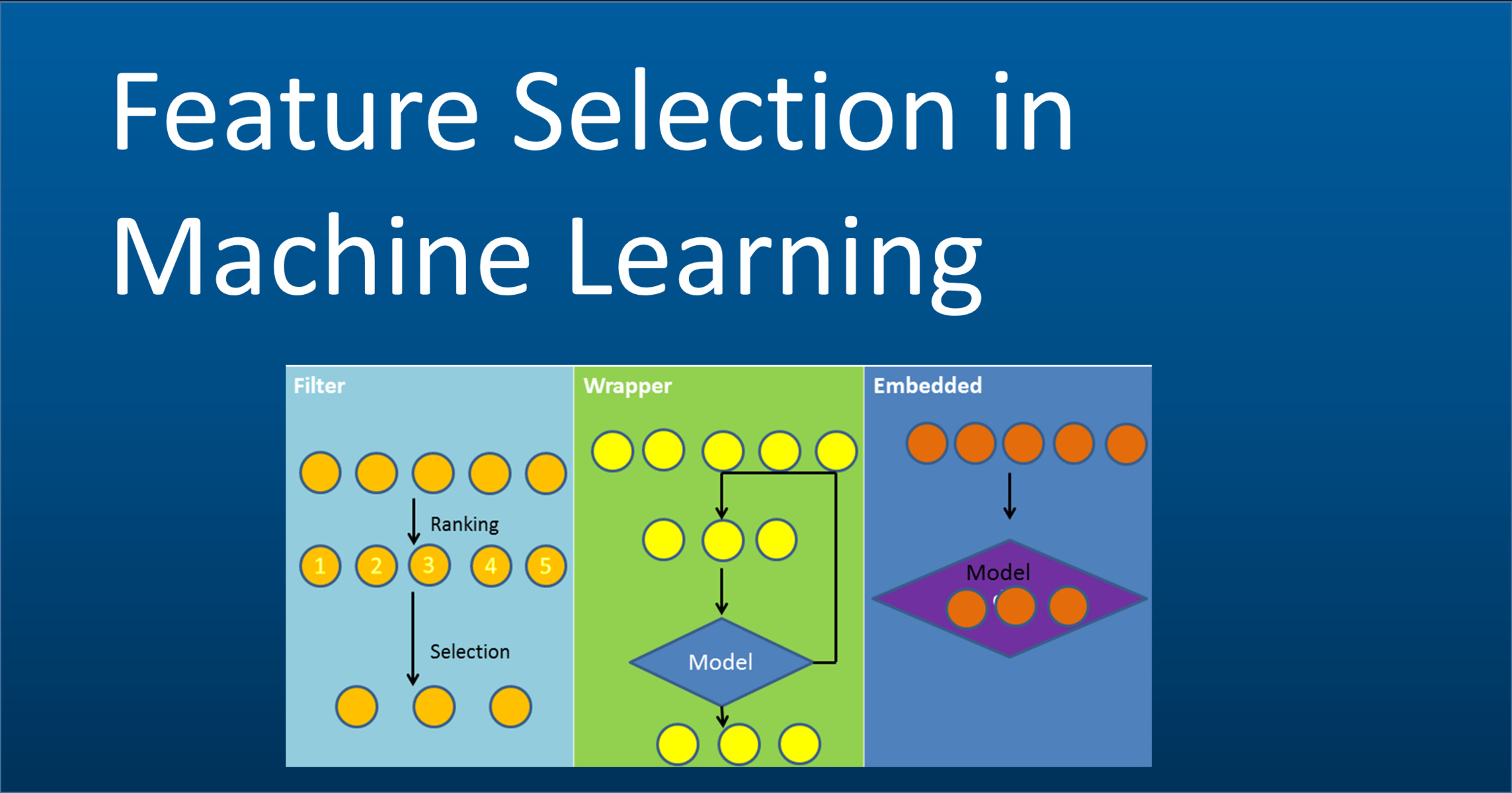
There are various techniques available for feature selection in machine learning, each with its strengths and limitations. Some common approaches include filter methods, wrapper methods, and embedded methods. Filter methods rely on statistical measures to evaluate the relevance of features, while wrapper methods use the model’s performance as a criterion. Embedded methods incorporate feature selection within the model’s training process.
In this article, we will explore different feature selection techniques and discuss their benefits and applications. By understanding these techniques, you will be equipped to make informed decisions when working with machine learning problems and optimize your models for better performance and interpretability.
What is Feature Selection?
Feature selection, also known as variable selection or attribute selection, is the process of identifying the subset of features that are most relevant to a given machine learning problem. In simpler terms, it involves choosing the most informative and discriminative features from a dataset to improve the performance and interpretability of a machine learning model.
Features, in the context of machine learning, are the input variables or attributes that represent the characteristics of the data. These features can include numeric values, categorical variables, or even text or image data. Feature selection helps to identify the subset of features that have the most influence on the target variable, while eliminating irrelevant or redundant features.
The need for feature selection arises when dealing with high-dimensional data, where the number of features exceeds the number of instances or observations. In such cases, including all available features in the model can lead to various issues, including overfitting, increased computational complexity, and reduced interpretability.
There are several reasons why feature selection is a critical step in the machine learning pipeline. Firstly, it helps to improve the model’s generalization ability by reducing the risk of overfitting. Overfitting occurs when a model learns to fit the training data too closely, resulting in poor performance on unseen data. By selecting the most relevant features, we reduce the chances of including noise or irrelevant information that can lead to overfitting.
Secondly, feature selection enhances the interpretability of the model. When a model contains a large number of features, it becomes challenging to understand the relationships between the predictors and the target variable. By selecting a subset of features, we can focus on the most important factors and gain insights into the underlying patterns and mechanisms driving the predictions.
Furthermore, feature selection can significantly improve the computational efficiency of the model. With fewer features, the training and prediction processes become faster, allowing us to work with large-scale datasets that would otherwise be computationally prohibitive.
Overall, feature selection is a crucial step in machine learning that involves the careful selection of the most relevant features to improve model performance, interpretability, and efficiency. By reducing the dimensionality of the dataset and focusing on the most informative attributes, we can enhance the accuracy, generalization, and efficiency of machine learning models.
Why is Feature Selection Important?
Feature selection plays a vital role in machine learning and data analysis due to its numerous benefits and impacts on model performance, interpretability, and computational efficiency. Let’s delve into why feature selection is important:
1. Mitigating the curse of dimensionality: The curse of dimensionality refers to the challenges that arise when working with high-dimensional datasets. Including all available features can lead to increased computational complexity, overfitting, and difficulty in interpreting the model. Feature selection helps overcome these challenges by reducing the dimensionality of the dataset and focusing on the most informative features.
2. Improving model performance: Including irrelevant or redundant features in a model can degrade its performance. Such features provide noisy or redundant information, leading to overfitting and poor generalization. By selecting the most relevant features, we enhance the model’s ability to distinguish between relevant and irrelevant patterns, resulting in improved performance on unseen data.
3. Enhancing model interpretability: A model with a large number of features can be challenging to interpret and understand. Feature selection allows us to focus on the most important and influential variables, providing insights into the underlying patterns and relationships between the predictors and the target variable. This interpretability is crucial for gaining trust and understanding in the decisions made by the model.
4. Reducing computational complexity: With an increasing number of features, the computational requirements of training and evaluating a model also increase. Selecting a subset of relevant features reduces the computational complexity, making it more feasible to work with large-scale datasets and reducing the time required for training and inference.
5. Handling multicollinearity: Multicollinearity occurs when there is a high correlation between two or more features. This can lead to numerical instability and difficulties in interpreting the model coefficients. Feature selection helps in identifying and excluding highly correlated features, improving the stability and interpretability of the model.
6. Dealing with noisy data: Datasets often contain noisy or irrelevant features that can negatively impact model performance. Feature selection eliminates these noisy features, allowing the model to focus on the most informative attributes and improving its ability to extract meaningful patterns from the data.
Overall, feature selection is of utmost importance in machine learning as it improves model performance, interpretability, and computational efficiency. By selecting the most relevant features, we can overcome the challenges of high-dimensional data, enhance the model’s ability to generalize, and gain insights into the underlying patterns and relationships within the data.
Types of Feature Selection Techniques
There are several approaches and techniques available for selecting the most informative features in a machine learning problem. These techniques can be broadly categorized into three main types: filter methods, wrapper methods, and embedded methods. Let’s explore each of these types in detail:
Filter Methods
Filter methods are feature selection techniques that rely on statistical measures to evaluate the relevance of features. These methods assess the intrinsic characteristics of the features and rank them based on their correlation with the target variable without considering the specific machine learning model being used.
Some commonly used filter methods include:
1. Pearson Correlation: This method measures the linear correlation between each feature and the target variable. Features with high correlation values are deemed more relevant and are selected for inclusion in the model.
2. Chi-Square: Chi-square measures the dependence between categorical features and the target variable. It is suitable for feature selection in classification problems where both the predictor and target variables are categorical.
3. Information Gain: Information Gain is a measure based on entropy that quantifies the amount of information provided by a feature towards predicting the target variable. Features with higher information gain are considered more important.
Wrapper Methods
Wrapper methods use the performance of the machine learning model as the evaluation criterion for feature selection. These methods explore different subsets of features by training and evaluating the model on various combinations to identify the optimal subset.
Some commonly used wrapper methods include:
1. Recursive Feature Elimination: This method starts with all features and iteratively removes the least important feature based on the model performance. It continues until a specified number of features or a performance threshold is reached.
2. Forward/Backward Selection: Forward selection starts with an empty set of features and adds one feature at each step based on the improvement in performance. Backward selection, on the other hand, starts with all features and eliminates one feature at each step based on performance degradation.
3. Genetic Algorithms: Genetic algorithms are optimization techniques inspired by the process of natural selection. These methods generate a population of feature subsets and select the best subsets based on their fitness measures evaluated using the model’s performance.
Embedded Methods
Embedded methods incorporate feature selection within the model training process itself. Instead of performing a separate feature selection step, these techniques optimize the feature subset during the model’s training process.
Some commonly used embedded methods include:
1. Lasso Regression: Lasso regression applies L1 regularization, which encourages sparsity in the coefficient vector. It promotes feature selection by shrinking less relevant features towards zero, effectively eliminating them from the model.
2. Ridge Regression: Ridge regression applies L2 regularization, which also penalizes the model for large coefficients but does not promote sparsity. It can help reduce the impact of irrelevant features but does not explicitly perform feature selection.
3. Decision Trees: Decision trees inherently perform feature selection by evaluating the importance of features in splitting the data at each node. Features that contribute more to the tree’s information gain or Gini impurity reduction are considered more important.
Each type of feature selection technique has its strengths and limitations, and the choice of method depends on the specific problem, dataset, and machine learning algorithm being used. A combination of multiple techniques may also be employed to achieve the best possible feature subset for a given problem.
Filter Methods
Filter methods are a popular type of feature selection techniques that evaluate the relevance of features based on intrinsic characteristics without considering the specific machine learning model being used. These methods rely on statistical measures to assess the relationship between each feature and the target variable. Let’s explore some commonly used filter methods:
1. Pearson Correlation:
Pearson correlation is a widely used measure to assess the linear relationship between two continuous variables. In the context of feature selection, it quantifies the correlation between each feature and the target variable. Features with a high absolute correlation coefficient are considered more relevant and are selected for inclusion in the model. Positive correlation indicates that as the feature value increases, the target variable tends to increase, and vice versa for negative correlation.
2. Chi-Square:
Chi-square is a measure of dependence between two categorical variables. It is commonly used for feature selection in classification problems where both the predictor and target variables are categorical. The Chi-square test compares the observed and expected frequencies of each feature-value combination and calculates a chi-square statistic. Higher values indicate stronger dependence between the feature and the target variable, making the feature more relevant for classification.
3. Information Gain:
Information Gain is a measure based on entropy that quantifies the amount of information provided by each feature towards predicting the target variable. It is often used for feature selection in decision tree-based algorithms. The idea behind Information Gain is to select features that yield the most significant reduction in uncertainty or entropy when their values are known. Features with higher Information Gain are considered more important as they contribute more towards predicting the target variable.
Filter methods have several advantages. They are computationally efficient since they consider the statistical relationship between features and the target variable independently of the model training process. Filter methods are also helpful when dealing with high-dimensional datasets or incomplete data where complex model assumptions may not hold. Furthermore, filter methods can provide insights into the individual relevance of features without requiring extensive computational resources.
However, a limitation of filter methods is that they do not consider the interactions or dependencies between features. They evaluate each feature in isolation, potentially overlooking important feature combinations that may be relevant in predicting the target variable. Additionally, filter methods may struggle when dealing with noisy or irrelevant features, as they are based solely on statistical measures and cannot account for the model’s inherent biases.
It’s important to note that filter methods should be used as a preliminary feature selection step to identify potentially relevant features. Subsequent steps, such as wrapper or embedded methods, can be employed to refine the feature subset based on the model’s predictive performance or specific requirements of the problem at hand.
By utilizing filter methods, data scientists can quickly and efficiently identify potentially relevant features and reduce the dimensionality of the dataset, laying the foundation for further analysis and model building.
Pearson Correlation
Pearson correlation is a widely used measure to assess the linear relationship between two continuous variables. In the context of feature selection, Pearson correlation evaluates the correlation between each feature and the target variable.
The Pearson correlation coefficient, commonly denoted as r, ranges from -1 to 1. A value close to 1 indicates a strong positive linear correlation, meaning that as the feature value increases, the target variable tends to increase as well. On the other hand, a value close to -1 indicates a strong negative linear correlation, with the target variable decreasing as the feature value increases. A value close to 0 suggests little to no linear correlation between the feature and the target variable.
When using Pearson correlation for feature selection, features with high absolute correlation coefficients are considered more relevant. The magnitude of the correlation coefficient represents the strength of the relationship, regardless of whether it is positive or negative. By selecting features with high correlation, we can identify the variables that have a strong influence on the target variable.
Pearson correlation is particularly useful when the relationship between the feature and the target variable is linear. If the relationship is nonlinear or exhibits complex patterns, the correlation coefficient may not accurately capture the strength of the relationship.
One important consideration when using Pearson correlation is that it only measures the linear relationship. It does not capture other types of relationships, such as quadratic or exponential dependencies. Therefore, it is crucial to complement Pearson correlation with other feature selection techniques that can capture nonlinear relationships, especially when working with non-linear machine learning algorithms.
Another limitation of Pearson correlation is that it only assesses the relationship between two variables in isolation. It does not consider the impact of other variables present in the dataset. Therefore, it may overlook important feature combinations that collectively provide valuable information for predicting the target variable. Considerations such as multicollinearity, where features may have high intercorrelations, should also be taken into account to avoid redundancy in the selected features.
Pearson correlation can be easily computed using standard statistical libraries, and it provides a quick way to assess the relevance of continuous features in linear modeling scenarios. By leveraging the insights gleaned from Pearson correlation, data scientists can identify the features that have the strongest influence on the target variable and prioritize them in model training and evaluation.
Chi-Square
Chi-square is a statistical measure that assesses the dependence between two categorical variables. In the context of feature selection, Chi-square evaluates the relationship between each categorical feature and the target variable, making it particularly suitable for classification problems.
The Chi-square test compares the observed and expected frequencies of each feature-value combination and calculates a statistic known as the chi-square statistic. A higher chi-square value indicates a stronger dependence between the feature and the target variable, suggesting that the feature is more relevant for classification.
To compute the chi-square statistic, we create a contingency table that displays the distribution of frequencies for each combination of feature values and target values. We then compare these observed frequencies with the frequencies we would expect if the feature and the target variable were independent.
If the observed frequencies are significantly different from the expected frequencies, the chi-square statistic will be large, indicating a strong dependence. On the other hand, if the observed frequencies closely match the expected frequencies, the chi-square statistic will be small, indicating little to no dependence.
Chi-square feature selection is particularly effective when both the predictor variable and the target variable are categorical. It allows us to identify the features that have a significant impact on the target variable and should be included in the model.
It’s important to note that Chi-square only evaluates the statistical dependence between variables and does not indicate the direction or nature of the relationship. Additionally, Chi-square assumes the independence of observations, which may not be true in all scenarios. Therefore, it is crucial to interpret the results of the Chi-square test alongside other considerations and domain knowledge.
In practice, Chi-square feature selection can be easily implemented using various statistical libraries. The output is typically a ranked list of features based on their chi-square statistic or related metrics such as p-values or information gain. By considering the Chi-square scores, data scientists can focus on the most relevant categorical features and improve the performance of their models when working with classification problems.
Information Gain
Information Gain is a measure based on entropy, a concept from information theory. It quantifies the amount of information provided by each feature towards predicting the target variable. Information Gain is commonly used as a feature selection criterion, especially in decision tree-based algorithms.
The concept of entropy measures the uncertainty or randomness in a set of data. In the context of feature selection, entropy represents the impurity of the target variable’s distribution. A feature with high Information Gain contributes the most towards reducing this impurity, making it more predictive of the target variable.
To calculate Information Gain, we first compute the entropy of the target variable before considering any split. Then, for each feature, we calculate the weighted average of the entropies of the target variable after splitting the data based on the feature’s values. The reduction in entropy achieved by the split is the Information Gain for that feature.
A higher Information Gain indicates that the feature provides more valuable information for predicting the target variable. Features with high Information Gain are deemed more relevant and are selected for inclusion in the model.
One advantage of Information Gain is that it can handle both categorical and numerical features and is not limited to a specific type of dataset. However, it performs best with discrete, categorical features that have a limited number of distinct values.
Information Gain is particularly effective when building decision tree-based models due to its ability to identify features that divide the data according to their class labels most effectively. Decision trees inherently perform feature selection by evaluating the importance of features in splitting the data at each node. Features that contribute more to the tree’s Information Gain or Gini impurity reduction are considered more important.
However, one limitation of Information Gain is that it tends to favor features with a large number of distinct values. Features with many distinct values may have high Information Gain simply due to their ability to split the data finely, even if the splitting is not truly meaningful or informative.
It’s worth noting that Information Gain is just one of several criteria used in decision tree-based algorithms, and different measures, such as Gini impurity, may produce different feature rankings. Additionally, Information Gain does not consider the interactions or combinations of features, which could be relevant in some scenarios.
Despite its limitations, Information Gain provides a powerful tool for feature selection in decision tree-based models and can help identify features that are most influential in predicting the target variable.
Wrapper Methods
Wrapper methods are a type of feature selection technique that utilizes the performance of a machine learning model as the evaluation criterion. These methods involve training and evaluating the model on different subsets of features to identify the optimal feature subset.
Wrapper methods explore different combinations of features by treating feature selection as a search problem. The goal is to find the subset of features that maximizes the predictive performance of the model. This evaluation is typically performed using cross-validation or other robust validation techniques to ensure the generalizability of the selected feature subset.
Some commonly used wrapper methods include:
1. Recursive Feature Elimination:
Recursive feature elimination (RFE) is a wrapper method that starts with all features and iteratively removes the least important feature based on the model’s performance. RFE assigns weights or rankings to each feature based on their importance and eliminates the least important ones at each iteration. This process continues until a specified number of features or a performance threshold is reached.
2. Forward/Backward Selection:
Forward selection starts with an empty set of features and iteratively adds one feature at each step based on the improvement in the model’s performance. Backward selection, on the other hand, starts with all features and eliminates one feature at each step based on performance degradation. These stepwise selection approaches continue until a stopping criterion is met, such as reaching a certain number of features or encountering a decline in performance.
3. Genetic Algorithms:
Genetic algorithms are search optimization techniques inspired by the process of natural selection. In the context of feature selection, genetic algorithms generate a population of feature subsets representing potential solutions. These subsets undergo genetic operations like selection, crossover, and mutation to produce new generations of feature subsets. The fitness of each subset is evaluated based on the model’s performance. The algorithm iterates until a satisfactory feature subset is found.
Wrapper methods have the advantage of considering the specific machine learning algorithm being used and the interactions between features. By directly evaluating the model’s performance, wrapper methods can capture the combined effect of multiple features and identify the optimal subset for a given model.
However, wrapper methods can be computationally expensive since they involve training the model multiple times for different feature subsets. Additionally, they may be prone to overfitting, especially when the feature space is large or the model is complex. Proper validation techniques, such as cross-validation, are crucial to ensure the selected feature subset’s generalizability.
Wrapper methods are particularly useful when the goal is to optimize the performance of a specific model and when the interactions between features are essential for accurate predictions. By systematically exploring different feature subsets, wrapper methods enable data scientists to uncover the most informative set of features that yield the best performance for the intended model.
Recursive Feature Elimination
Recursive Feature Elimination (RFE) is a wrapper method for feature selection that aims to identify the most relevant set of features by recursively eliminating the least important features based on the performance of a machine learning model. RFE assigns weights or rankings to each feature and iteratively removes the features with the lowest weights.
The RFE process starts with all the features and trains a model using the entire feature set. The feature importance is then assessed, either directly through model-specific coefficients or indirectly using feature selection techniques like filtering methods. Based on the importance scores, the least important feature(s) are discarded. The model is retrained on the remaining features and the process is repeated until the desired number of features or a stopping criterion is reached.
By iteratively eliminating features, RFE helps to find the subset of features that contributes the most to the model’s performance. It aims to strike a balance between simplicity and accuracy, as removing irrelevant or redundant features can reduce overfitting and improve interpretability while preserving crucial information for accurate predictions.
RFE’s strength lies in its ability to consider feature interactions. Since each iteration trains the model on an updated feature set, RFE implicitly captures the impact of feature combinations. This makes it particularly beneficial when features exhibit non-linear or complex interactions that affect the model’s performance.
One popular usage of RFE is in conjunction with linear models like linear regression or support vector machines, where the feature coefficients can serve as importance measures. Starting with a full set of features, RFE eliminates the least significant feature(s) based on their coefficients. This process continues until the desired number of features or a specified performance threshold is achieved.
RFE is a flexible feature selection technique that can be adapted to different models and evaluation metrics. It allows data scientists to systematically explore the feature space and obtain an optimal subset of features for their specific modeling objectives.
However, RFE does have some considerations. It can be computationally intensive, particularly when working with a large number of features or a complex model. The performance of RFE heavily relies on the model’s sensitivity to feature elimination, which can vary depending on the algorithm and the dataset. Additionally, the optimal number of features to retain may require experimentation and tuning.
Overall, Recursive Feature Elimination provides a valuable approach to feature selection, offering a systematic way to identify the most relevant features in a recursive manner. Its ability to account for feature interactions makes it a powerful tool in various machine learning problems.
Forward/Backward Selection
Forward/Backward selection is a wrapper method for feature selection that aims to find the most relevant subset of features by iteratively adding or removing features based on the performance of a machine learning model. This approach is commonly used when the goal is to build a predictive model using a subset of the available features.
Forward selection starts with an empty set of features and iteratively adds one feature at each step based on the improvement in the model’s performance. At each iteration, the model is trained and evaluated on the existing set of features plus one additional candidate feature. The feature that leads to the largest performance improvement is selected and retained for the next iteration. This process continues until a specified number of features or a stopping criterion is reached.
On the other hand, backward selection starts with all features and iteratively removes one feature at each step based on the degradation in the model’s performance. At each iteration, the model is trained and evaluated on the existing set of features minus one feature. The feature that results in the smallest performance degradation is eliminated, and the process continues until the desired number of features or a stopping criterion is met.
Both forward and backward selection methods aim to find the optimal feature subset by considering the interdependencies between features and their impact on the model’s performance. By iteratively evaluating the model with different feature combinations, these methods provide a systematic approach to feature selection.
Forward selection starts with a small set of features and progressively adds features that contribute the most to the model’s performance. This approach guarantees that the retained features are the ones that individually enhance the model’s predictive power the most. However, forward selection may not consider interactions between features that could be important for accurate predictions. It may overlook subsets of features that collectively provide valuable information.
Backward selection, on the other hand, starts with all features and eliminates features that have the least impact on the model’s performance. This approach allows for the consideration of feature interactions, as the impact of removing one feature accounts for the effect of that feature in combination with the other features. However, backward selection may suffer from the increased risk of eliminating features prematurely, as the removal of one feature can influence the relevance of other features.
Both forward and backward selection methods require careful consideration of stopping criteria to avoid overfitting or underfitting the model. Common criteria include a predefined number of features, reaching a desired performance threshold, or observing degradation in performance after feature addition or removal.
Forward/Backward selection provides a flexible approach to feature selection that accounts for the interplay between features and their impact on model performance. By iteratively evaluating different feature combinations, data scientists can identify the most relevant subset of features for their specific prediction task.
Genetic Algorithms
Genetic Algorithms (GAs) are a type of wrapper method for feature selection that is inspired by the process of natural selection and evolution. GAs utilize principles from genetics and evolution to search for the most relevant subset of features that optimize the performance of a machine learning model.
The process starts by generating an initial population of feature subsets, where each individual subset represents a potential solution. Each individual is evaluated based on a fitness measure, which is typically the performance of the model using the selected features. Individuals with higher fitness values are more likely to be selected for further iterations.
Reproduction involves selecting the fittest individuals and applying genetic operations, such as crossover and mutation, to create offspring. Crossover combines the genetic information of two parent feature subsets, while mutation introduces small, random changes to maintain diversity in the population. The offspring then undergo evaluation, and the process continues for several generations, allowing the fittest individuals to evolve and potentially reach an optimal feature subset.
The iterative nature of genetic algorithms helps explore the search space of feature combinations. By evaluating the fitness of each individual, the algorithm identifies and promotes feature subsets that contribute most to the performance of the model. Over time, the algorithm tends to converge towards a subset of features that exhibits superior performance.
Genetic algorithms are particularly useful when the search space of all possible feature subsets is vast and exhaustive methods become computationally infeasible. Unlike exhaustive search techniques, genetic algorithms offer a trade-off between exploration and exploitation of the search space, allowing for efficient feature selection.
One advantage of genetic algorithms is their ability to account for feature interactions and dependencies. Crossover operations enable the recombination of subsets, allowing information from different individuals to be combined. This helps consider potential interactions between features that are crucial for accurate predictions.
However, genetic algorithms come with some considerations. They can be computationally expensive, especially when the search space is large and the evaluation of fitness requires training and evaluating the model multiple times. They also require careful tuning of parameters, such as crossover rate and mutation rate, to strike a balance between exploration and exploitation.
With their ability to systematically explore the feature space and account for feature interactions, genetic algorithms offer a powerful method for feature selection. They allow data scientists to discover feature subsets that optimize model performance and provide insights into the most informative features for a given prediction problem.
Embedded Methods
Embedded methods are a type of feature selection technique that integrates feature selection within the model training process itself. These methods incorporate feature selection as an inherent part of the model building process, ensuring that the selected features are optimized for the specific machine learning algorithm being used.
Embedded methods have the advantage of considering the interaction between features and the model’s objective function. By incorporating feature selection within the training process, these methods can identify the most relevant features that contribute to the model’s performance and improve its accuracy and efficiency.
Here are some commonly used embedded methods:
1. Lasso Regression:
Lasso regression (Least Absolute Shrinkage and Selection Operator) is a linear regression model that applies L1 regularization. Lasso regression optimizes the model’s objective function by penalizing the magnitude of the coefficients. This penalty encourages sparsity in the coefficient vector, resulting in some coefficients being shrunk towards zero. Features with non-zero coefficients are considered selected. Lasso regression effectively performs feature selection by retaining only the most relevant features.
2. Ridge Regression:
Ridge regression is a linear regression model that applies L2 regularization. Unlike Lasso regression, which promotes sparsity, Ridge regression penalizes the magnitude of the coefficients without explicitly promoting sparsity. While it does not perform feature selection by eliminating features, it can help reduce the impact of irrelevant or noisy features by shrinking their coefficients towards zero. Ridge regression is useful when the goal is to reduce multicollinearity and stabilize the model’s performance.
3. Decision Trees:
Decision trees inherently perform feature selection during the training process. At each node, a decision tree algorithm selects the feature that provides the most information gain or the most significant reduction of impurity (e.g., Gini impurity). The features that contribute more to splitting the data are considered more important. By prioritizing features that provide the most discriminatory power, decision trees effectively select relevant features during their construction.
Embedded methods have the advantage of being model-specific and tailored to the machine learning algorithm being used. They automatically consider interactions between features and optimize the feature subset based on the model’s objective function.
However, embedded methods also come with some considerations. They may not be suitable for all machine learning algorithms, as some algorithms already have inherent feature selection mechanisms. Additionally, the effectiveness of embedded methods depends heavily on the quality of the training dataset and the model’s representation capacity.
Overall, embedded methods provide a powerful approach to feature selection, as they integrate the feature selection process within the model training process. By selecting features that are optimized for the model’s objective, these methods can enhance model performance, improve interpretability, and reduce computational complexity.
Lasso Regression
Lasso regression (Least Absolute Shrinkage and Selection Operator) is a linear regression model that incorporates regularization using L1 penalty. This regularization technique promotes sparsity in the coefficient vector, effectively performing feature selection. Lasso regression is highly effective in situations where the number of predictors is high compared to the number of observations.
The L1 penalty in Lasso regression encourages some of the coefficient values to be exactly zero, resulting in sparse models that only include the most important features. By shrinking some coefficients to zero, Lasso regression effectively performs feature selection by discarding irrelevant or redundant features from the model.
Through the L1 regularization term, Lasso regression balances the trade-off between model complexity and prediction accuracy. The regularization term penalizes large coefficient values, forcing less important features to have close to zero coefficients. In contrast, features that are deemed important by the model tend to have non-zero coefficients, indicating their relevance in predicting the target variable.
When fitting a Lasso regression model, an important hyperparameter to consider is the strength of the regularization, also known as the regularization parameter (λ or alpha). Higher values of λ result in more aggressive shrinking of the coefficients, leading to sparser models with fewer selected features. Lower values of λ preserve more features, potentially increasing model complexity but also capturing more intricate relationships.
Lasso regression is particularly useful in scenarios where feature selection and model interpretability are paramount. By automatically identifying and selecting important features, Lasso regression simplifies the model and improves interpretability. It allows for a concise understanding of the most influential predictors and the relationships between them and the target variable.
One important consideration when using Lasso regression is the potential for multicollinearity. If highly correlated features exist in the dataset, Lasso regression may arbitrarily select one feature and shrink the coefficients of the others towards zero, even if they are individually important. To address this, careful preprocessing steps, such as data transformation or feature grouping, might be necessary.
Lasso regression can effectively handle high-dimensional datasets and identify the most relevant features for a specific prediction problem. Its ability to perform variable selection while maintaining prediction accuracy makes it a valuable tool in various domains, including finance, genetics, and social sciences.
Ridge Regression
Ridge regression is a linear regression model that incorporates regularization using L2 penalty. It is similar to Lasso regression but with a different regularization term. The L2 penalty in Ridge regression reduces the magnitude of the coefficients without explicitly promoting sparsity. Instead, Ridge regression aims to reduce the impact of irrelevant or noisy features while preserving all predictors in the model.
Ridge regression adds the squared sum of the coefficients multiplied by a regularization parameter (λ or alpha) to the loss function. This penalty encourages the model to distribute the coefficient values more evenly and shrink them towards zero. However, unlike Lasso regression, Ridge regression typically does not lead to exact zero coefficients, even for unimportant features.
The L2 regularization term in Ridge regression provides several benefits. Firstly, it helps mitigate the issue of multicollinearity, which occurs when predictors are highly correlated. By shrinking the coefficient values, Ridge regression reduces the sensitivity of the model to collinear features, stabilizing the estimates and improving prediction performance.
Secondly, Ridge regression can improve the generalization ability of the model by reducing overfitting. The regularization term controls the model complexity, preventing the coefficients from becoming too large and limiting the model’s flexibility. This regularization can lead to better performance when the dataset has noise or when the number of predictors is large compared to the number of observations.
In contrast to Lasso regression, Ridge regression does not explicitly perform variable selection. It aims to retain all predictors while minimizing their impact by constraining the coefficients. This can be advantageous when complete feature information is desired or when it is important to maintain the interpretability of the model.
The choice of the regularization parameter (λ or alpha) in Ridge regression is crucial. A larger value of the regularization parameter increases the amount of shrinkage, resulting in smaller coefficient values. As the regularization parameter approaches zero, the Ridge regression model becomes closer to ordinary linear regression without regularization.
Ridge regression should be considered when there is a need to reduce multicollinearity, stabilize the model’s performance, and maintain all predictors in the model. It is also commonly used when the predictors are all potentially relevant and there is no strong prior belief about which features should be excluded.
Overall, Ridge regression provides a regularization technique that balances the trade-off between prediction accuracy and model complexity. By promoting smoother and more stable coefficient estimates, Ridge regression is a valuable tool for addressing collinearity and improving the performance of linear regression models.
Decision Trees
Decision trees are a popular class of machine learning algorithms that naturally perform feature selection as part of their training process. These algorithms are particularly effective when it comes to handling both categorical and numerical features and can handle complex datasets with non-linear relationships.
At each node of a decision tree, a splitting criterion is used to assess the importance of features in determining the target variable. The feature that provides the most discriminatory power, typically measured by information gain or Gini impurity reduction, is selected to split the data. By prioritizing features that contribute the most to the decision-making process, decision trees inherently perform feature selection during their construction.
The nature of decision trees allows them to capture intricate relationships and interactions between features. The split decisions made by decision trees can involve multiple features, uncovering patterns that involve combinations of predictors. This feature interaction detection is crucial for accurate predictions, especially in domains where feature combinations have a strong influence on the target variable.
Decision trees have several advantages when it comes to feature selection. Firstly, the feature-importance ranking provided by a decision tree algorithm can easily identify the most influential features in the dataset. These important features can then be used for further analysis or model construction.
Secondly, decision trees can handle both continuous and categorical features without requiring extensive preprocessing or explicit encoding. This makes them versatile in working with different types of datasets.
However, decision trees can be prone to overfitting, especially when they are allowed to grow deeper and capture noise in the training data. Overfitting can result in the selection of irrelevant features and reduced generalization performance on new, unseen data. To address this, techniques like pruning, ensemble methods (e.g., random forests), or setting depth limits can be employed to control model complexity and improve generalization.
Another consideration with decision trees is their sensitivity to small changes in the dataset. Decision trees are not robust to variations in the training data, and even slight perturbations can lead to different feature selections. Thus, it is important to evaluate feature importance across multiple runs or apply ensemble methods that aggregate the results of multiple decision trees.
Overall, decision trees provide an intuitive and powerful approach to feature selection. By inherently evaluating feature importance during their construction, decision trees can identify the most relevant features and capture complex relationships in the data. Their ability to handle mixed feature types and detect feature interactions makes them widely used and effective in a variety of machine learning problems.
Evaluating Feature Selection
The effectiveness of feature selection techniques is a crucial aspect that needs to be evaluated to ensure the quality of the selected feature subset. Evaluating feature selection can provide insights into the impact of the selected features on the model’s performance, interpretability, and generalizability.
One common approach to evaluating feature selection is by comparing the performance of the model with and without feature selection. This comparison is typically done using appropriate evaluation metrics such as accuracy, precision, recall, F1-score, or area under the receiver operating characteristic curve (AUC-ROC). These metrics help assess the model’s performance and determine whether feature selection has improved or negatively impacted the model’s ability to make accurate predictions.
In addition to performance metrics, it is essential to evaluate the stability and robustness of the selected feature subset. Stability refers to the consistency of the selected features when the feature selection process is repeated with different subsets of the data or using different models. Robustness refers to the ability of the selected features to generalize well to new, unseen data. Cross-validation or bootstrap resampling techniques can be employed to assess stability and robustness.
Moreover, evaluating feature selection should also consider the interpretability and practicality of the selected features. Models with a reduced set of features are often more easily interpretable and allow for a better understanding of the underlying patterns. Domain experts can analyze the selected features to gain insights into the problem domain and validate the relevance of the selected features.
Beyond performance and interpretability, it is crucial to assess the computational aspects of feature selection. Some feature selection techniques can be computationally expensive, especially when dealing with high-dimensional datasets. The time and resource requirements should be taken into account to ensure the feasibility of applying the selected technique in practice.
Lastly, proper evaluation of feature selection techniques may involve comparing different feature selection methods, either within the same category or across different types of techniques. This comparison can help identify the strengths and limitations of each method and choose the most appropriate approach for the specific problem and dataset.
Overall, evaluating feature selection involves assessing the impact of the selected features on model performance, stability, interpretability, and practicality. By thoroughly evaluating the effectiveness of feature selection techniques, data scientists can make informed decisions about the relevance and utility of the selected feature subset for the given machine learning problem.
Conclusion
Feature selection is a critical step in machine learning that involves identifying the most relevant and informative features for a given prediction task. By selecting the appropriate subset of features, we can improve model performance, interpretability, and computational efficiency.
Throughout this article, we explored various types of feature selection techniques. Filter methods utilize statistical measures to assess feature relevance, including Pearson correlation, Chi-square, and Information Gain. Wrapper methods incorporate the model’s performance as the evaluation criterion, such as Recursive Feature Elimination, Forward/Backward Selection, and Genetic Algorithms. Embedded methods integrate feature selection within the model training process, including Lasso Regression, Ridge Regression, and Decision Trees.
Each technique has its strengths and limitations, and the choice of method depends on the specific problem, the dataset, and the machine learning algorithm being used. It is important to consider the trade-offs between model performance, interpretability, computational complexity, and the specific requirements of the problem at hand.
When evaluating feature selection, it is crucial to assess the impact of the selected features on model performance, stability, interpretability, and practicality. Performance metrics, stability analysis, interpretability validation by domain experts, and computational considerations all contribute to the comprehensive evaluation of feature selection techniques.
By employing effective feature selection techniques, data scientists can improve their models’ accuracy, interpretability, and efficiency. Feature selection aids in identifying the subset of features that have the most significant impact on the prediction task, resulting in more effective and reliable machine learning models.