Introduction
When it comes to machine learning algorithms, one commonly used method for binary classification is logistic regression. Logistic regression is a statistical technique that allows us to predict the probability of an event occurring based on given input variables. While the name might suggest a connection to regression analysis, logistic regression is actually a classification algorithm.
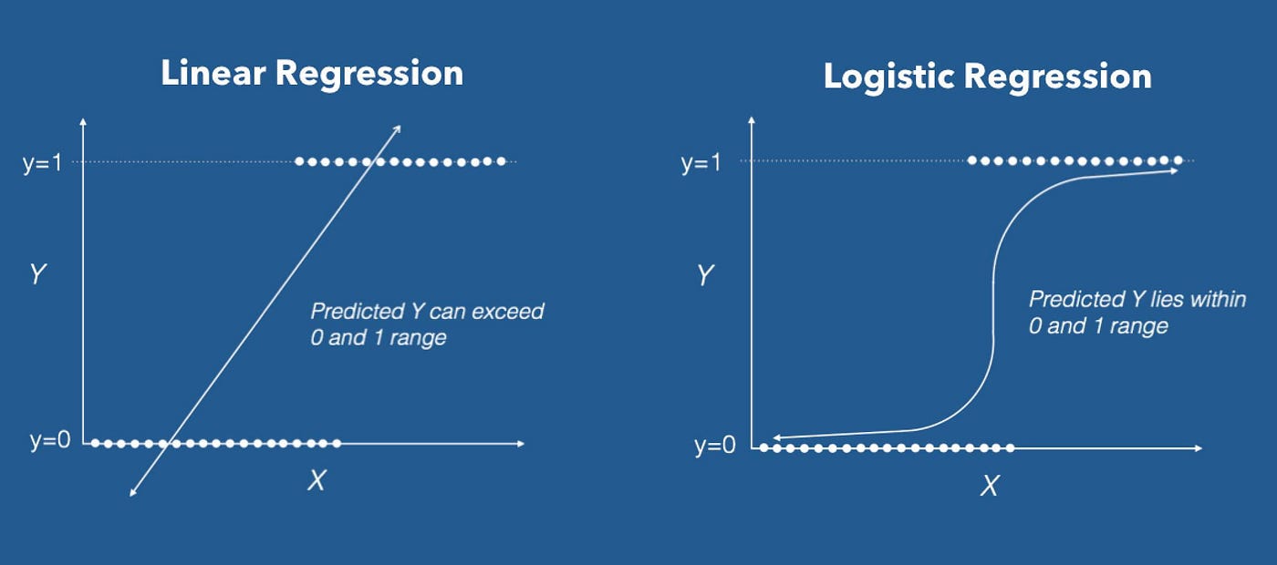
Unlike linear regression, which predicts continuous numerical values, logistic regression is employed when we want to classify instances into discrete categories. For example, it can be used to predict whether a customer will churn or not, whether an email is spam or not, or whether a patient will develop a certain disease or not. With logistics regression, we can model the relationship between a set of independent variables and the probability of a binary outcome.
Logistic regression is popular among machine learning practitioners due to its simplicity and efficiency. It doesn’t require a large amount of computational resources compared to other algorithms, making it suitable for handling large datasets. Moreover, it provides interpretable results, allowing us to understand the impact of different input variables on the outcome.
In this article, we will delve into the details of logistic regression, understanding the mathematical intuition behind it, the key components that drive its functionality, and the steps involved in training and evaluating a logistic regression model. We will also explore the pros and cons of logistic regression.
Whether you are new to machine learning or already familiar with other techniques, understanding logistic regression is a valuable asset for your data analysis toolbox. So, let’s dive in and uncover the essence of logistic regression and its practical applications.
Overview of Logistic Regression
Logistic regression is a statistical algorithm used for binary classification tasks. It allows us to predict the probability of an event occurring based on given input variables. The goal is to find the best-fitting curve that separates the two classes and predicts the probability of each class.
In logistic regression, the dependent variable is categorical, taking on two values, typically represented as 0 or 1. The independent variables, also known as features, can be numerical or categorical. These features are used to estimate the probability of the dependent variable taking on the value of 1.
One of the key assumptions in logistic regression is that the relationship between the independent variables and the logarithm of the odds is linear. The log-odds, also known as the logits, are transformed using a sigmoid function to map the predicted values to probabilities.
The logistic regression model can be represented by the equation:
y = β0 + β1x1 + β2x2 + … + βnxn
where y is the dependent variable, β’s are the coefficients or weights associated with each feature x, and n is the total number of features.
To train a logistic regression model, we use a technique called maximum likelihood estimation (MLE). The goal is to find the set of coefficients that maximizes the likelihood of observing the given data. This involves iteratively adjusting the weights using an optimization algorithm such as gradient descent until the model converges.
Once the model is trained, we can use it to make predictions on new data. The predicted probabilities can be transformed into class labels by applying a decision threshold. For example, if the predicted probability is greater than 0.5, we can classify the instance as belonging to the positive class; otherwise, it belongs to the negative class.
Logistic regression has several advantages, such as its simplicity and interpretability. It allows us to understand the impact of each feature on the predicted probabilities. However, logistic regression also has limitations. It assumes a linear relationship between the features and the log-odds, which may not always hold. Additionally, logistic regression is not suitable for problems with highly nonlinear relationships.
In the next section, we will explore the mathematical intuition behind logistic regression and how it handles probabilities and odds.
Mathematical Intuition
Understanding the mathematical intuition behind logistic regression is key to grasping its underlying principles. At the heart of logistic regression is the concept of probabilities and odds. Let’s explore these in more detail.
Probabilities: In logistic regression, we aim to estimate the probability of an event occurring. Probability values range from 0 to 1, with 0 indicating the event is impossible and 1 indicating the event is certain. For binary classification, we are interested in the probability of the event belonging to one of the two classes.
Odds: Odds represent the ratio of the probability of an event occurring to the probability of it not occurring, or in other words, the likelihood of success versus failure. The odds can range from 0 to infinity. For example, if the probability of an event is 0.8, the odds would be 0.8 / (1 – 0.8) = 4, indicating that the event is 4 times more likely to occur than not.
Now, how do we convert these probabilities and odds into a linear relationship suitable for logistic regression?
Logit Transformation: In logistic regression, we take the logarithm of the odds, known as the logit transformation, to ensure the relationship between the independent variables and the dependent variable is linear. The logit function can be defined as:
logit(p) = log(p / (1 – p))
where p is the probability of the event occurring. By taking the logarithm, we map the probabilities to a continuous range, allowing for a linear relationship between the independent variables and the log-odds.
Sigmoid Function: To map the logit-transformed values back to probabilities, we use a sigmoid function, also known as the logistic function. The sigmoid function can be represented as:
f(z) = 1 / (1 + e-z)
where z is the linear combination of the independent variables and their corresponding weights. The sigmoid function ensures that the predicted probabilities are bounded between 0 and 1, facilitating binary classification.
Decision Boundary: The decision boundary in logistic regression is the threshold that determines whether an instance belongs to one class or another. By default, the decision threshold is set at 0.5. If the predicted probability is greater than 0.5, the instance is classified as belonging to the positive class; otherwise, it belongs to the negative class.
In the next section, we will delve into the cost function used in logistic regression and the optimization algorithm called gradient descent.
Probability and Odds
In logistic regression, we deal with probabilities and odds to estimate the likelihood of an event occurring. Understanding the concepts of probabilities and odds is essential for comprehending logistic regression’s mathematical foundation.
Probability is a measure of the likelihood of an event occurring. In logistic regression, we are interested in the probability of an instance belonging to a specific class. The probability values range from 0 to 1, where 0 indicates the event is impossible, and 1 indicates the event is certain. For binary classification, we calculate the probability of the event belonging to one of the two classes.
Odds, on the other hand, represent the ratio of the probability of an event occurring to the probability of it not occurring. It is a measure of the likelihood of success compared to failure. The odds can range from 0 to infinity. For instance, if a customer has a 0.8 probability of purchasing a product, the odds of them purchasing the product would be 0.8 / (1 – 0.8) = 4, indicating that they are four times more likely to purchase the product than not.
Now, how do we convert these probabilities and odds into a form suitable for logistic regression?
In logistic regression, we employ the logit transformation to establish a linear relationship between the independent variables and the dependent variable. The logit function, denoted as logit(p), is defined as the logarithm of the odds:
logit(p) = log(p / (1 – p))
By taking the logarithm of the odds, we transform the probabilities into a continuous range, making it possible to model the relationship with the independent variables using linear regression.
To map the logit-transformed values back to probabilities, we use a sigmoid function, also known as the logistic function. The sigmoid function can be represented as:
f(z) = 1 / (1 + e-z)
Here, z represents the linear combination of the independent variables and their corresponding weights. The sigmoid function ensures that the predicted probabilities fall within the range of 0 to 1, which is necessary for binary classification.
Understanding the concepts of probabilities and odds in logistic regression provides the foundation for interpreting the predicted probabilities and making classification decisions based on a given threshold. In the next section, we will explore the sigmoid function and how it relates to the decision boundary in logistic regression.
Sigmoid Function
In logistic regression, the sigmoid function plays a crucial role in mapping the linear combination of independent variables to a probability value. The sigmoid function is also known as the logistic function due to its characteristic S-shaped curve.
The sigmoid function, denoted as f(z), is defined as:
f(z) = 1 / (1 + e-z)
Here, z represents the linear combination of the independent variables and their corresponding weights in the logistic regression model. The sigmoid function takes this linear combination and transforms it into a probability value.
The sigmoid function ensures that the predicted probabilities fall within the range of 0 to 1. As the value of z increases, the sigmoid function approaches 1, indicating a higher probability. Conversely, as the value of z decreases, the sigmoid function approaches 0, indicating a lower probability. The midpoint of the S-curve, which occurs at z = 0, corresponds to a probability of 0.5.
The sigmoid function’s shape is crucial in logistic regression because it allows us to make binary classifications based on a decision threshold. By default, the decision threshold is set at 0.5. If the predicted probability is greater than 0.5, the instance is classified as belonging to the positive class. If the predicted probability is less than or equal to 0.5, the instance is classified as belonging to the negative class.
It’s important to note that the sigmoid function is differentiable, which is essential for the training of logistic regression models using optimization algorithms such as gradient descent. The derivative of the sigmoid function can be computed easily, enabling the calculation of gradients and the refinement of model parameters.
The sigmoid function’s ability to map the linear combination of independent variables to a probability value makes logistic regression a versatile algorithm for binary classification tasks. However, it is worth noting that the sigmoid function assumes a specific form for the relationship between the variables and the probabilities. In cases where the relationship is highly nonlinear, alternative models such as nonlinear regression or decision trees may be more appropriate.
In the next section, we will explore the concept of the decision boundary and how logistic regression uses it for classification.
Decision Boundary
In logistic regression, the decision boundary is a critical concept that determines how instances are classified into different classes. It is the threshold or dividing line that separates the positive class from the negative class.
The decision boundary is based on the predicted probabilities generated by the logistic regression model. By default, the decision threshold is set at 0.5. If the predicted probability for an instance is greater than 0.5, it is classified as belonging to the positive class. If the predicted probability is less than or equal to 0.5, it is classified as belonging to the negative class.
For example, suppose we are using logistic regression to predict whether a customer will churn (1) or not (0) based on their past behavior. If the predicted probability of churn for a particular customer is 0.7, which is greater than the decision threshold of 0.5, we classify that customer as likely to churn. Conversely, if the predicted probability is 0.3, below the decision threshold, we classify the customer as likely to stay.
The decision boundary is determined by the logistic regression model’s parameters, including the weights assigned to the features. These weights indicate the relative importance of each feature in predicting the outcome. The decision boundary can be linear or nonlinear, depending on the relationship between the features and the predicted probabilities.
In the case of linear logistic regression, the decision boundary is a straight line or hyperplane that separates the two classes. If we have two features, the decision boundary is a straight line on a two-dimensional graph. In higher dimensions, it becomes a hyperplane.
However, in cases where the relationship between the features and the probabilities is nonlinear, the decision boundary can be nonlinear as well. This flexibility allows logistic regression to capture complex relationships and make accurate predictions in a wide range of scenarios.
It’s important to note that the decision boundary is sensitive to the decision threshold. By adjusting the threshold, we can control the trade-off between false positives and false negatives. A lower threshold results in more instances being classified as positive, which could lead to a higher false positive rate. Conversely, a higher threshold increases the false negative rate.
Understanding the concept of the decision boundary in logistic regression helps us interpret the classification results and evaluate the model’s performance. In the next section, we will explore the cost function used in logistic regression and the optimization algorithm called gradient descent.
Cost Function
In logistic regression, the cost function is used to measure the performance of the model and guide the optimization process. The goal is to find the set of model parameters that minimizes the cost function, resulting in the most accurate predictions. Typically, the cost function used in logistic regression is known as the log-loss or binary cross-entropy.
The log-loss function takes into account the difference between the predicted probabilities and the actual class labels. It penalizes the model for incorrect predictions by assigning a higher cost for instances that are misclassified.
Let’s denote the predicted probability for a positive class instance as p and the corresponding actual class label as y. The log-loss function can be defined as:
cost(p, y) = -y * log(p) – (1 – y) * log(1 – p)
When the actual class label y is 1, the second term (1 – y) * log(1 – p) becomes zero. Similarly, when y is 0, the first term -y * log(p) becomes zero. This way, the cost function provides a measure of the prediction accuracy for each individual instance.
To evaluate the performance of the entire logistic regression model, we calculate the average cost over all instances in the training dataset. The goal during the training phase is to find the set of model parameters that minimizes this average cost.
One popular optimization algorithm used to minimize the cost function in logistic regression is gradient descent. Gradient descent iteratively adjusts the model’s parameters by taking small steps in the direction of steepest descent. In each iteration, the gradients of the cost function with respect to the model parameters are computed. These gradients indicate the direction for updating the weights to reduce the cost. The process continues until convergence is achieved, and the cost function is minimized.
The choice of a suitable learning rate is crucial in gradient descent. A learning rate that is too small may result in slow convergence, while a learning rate that is too large may cause the algorithm to overshoot the minimum. It is common to experiment with different learning rates and monitor the cost function’s behavior during training to ensure an optimal balance.
The cost function, along with the optimization algorithm, plays a key role in training the logistic regression model and finding the optimal set of parameters. By minimizing the cost, the model learns to make accurate predictions and separate the different classes effectively.
In the next section, we will explore the evaluation techniques used to assess the performance of a logistic regression model.
Gradient Descent
Gradient descent is an optimization algorithm commonly used in logistic regression to minimize the cost function and find the optimal set of model parameters. It iteratively adjusts the weights until convergence, resulting in a model that accurately predicts the probability of the positive class.
The process of gradient descent starts with initializing the model’s parameters randomly or with certain predefined values. The cost function is then calculated based on these initial parameters. The algorithm aims to find the minimum of the cost function by iteratively updating the weights and calculating the cost function at each step.
The update of the weights is determined by the gradients of the cost function with respect to the model’s parameters. The gradient represents the direction of steepest ascent in the parameter space. In each iteration, the weights are adjusted in the opposite direction of the gradient, reducing the cost function.
The learning rate, often denoted as α, controls the step size taken in each iteration. A small learning rate may result in slow convergence, while a large learning rate can cause the algorithm to overshoot the minimum and potentially diverge. Finding the optimal learning rate is crucial for efficient convergence.
The gradient descent algorithm updates the weights using the following equation:
new_weight = old_weight – α * gradient
The gradient is calculated by taking the partial derivatives of the cost function with respect to each weight. The mathematical computation of the gradient depends on the specific form of the cost function used in logistic regression.
As the iterations progress, the weights are adjusted in the direction that minimizes the cost function, leading to a more accurate logistic regression model. The algorithm continues until convergence is reached, typically defined by a specified threshold or when the change in the cost function value becomes negligible.
Gradient descent is an iterative process that can require a large number of iterations, especially for complex datasets or when the learning rate is small. However, it is a powerful optimization algorithm that is widely used in logistic regression due to its effectiveness and simplicity.
It is important to note that there are variations of gradient descent, such as stochastic gradient descent and mini-batch gradient descent, which use different sampling techniques to update the weights. These variations can improve the efficiency of the algorithm and handle large datasets more effectively.
In the next section, we will explore the evaluation techniques used to assess the performance of a logistic regression model.
Evaluating the Model
Once a logistic regression model is trained, it is essential to evaluate its performance to determine its effectiveness in making predictions. Several evaluation techniques can be used to assess the model’s accuracy and generalization capabilities.
Confusion Matrix: A confusion matrix is a table that summarizes the performance of a classification model. It provides a detailed breakdown of the predicted and actual class labels, indicating the number of true positives, true negatives, false positives, and false negatives. From the confusion matrix, metrics such as accuracy, precision, recall, and F1 score can be calculated.
Accuracy: Accuracy measures the overall correctness of the model’s predictions and is calculated by dividing the number of correctly classified instances by the total number of instances. While accuracy is a useful metric, it might not be sufficient if the classes are imbalanced.
Precision and Recall: Precision measures the proportion of true positive predictions out of the instances classified as positive. It focuses on the accuracy of positive predictions. Recall, on the other hand, measures the proportion of true positive predictions out of the actual positive instances. It focuses on the model’s ability to identify positive instances correctly.
F1 Score: The F1 score is the harmonic mean of precision and recall, providing a balance between the two metrics. It ranges from 0 to 1, with 1 being the best score. The F1 score is particularly useful when the classes are imbalanced.
Receiver Operating Characteristic (ROC) Curve: The ROC curve is a graphical representation of the model’s performance. It plots the true positive rate (TPR) against the false positive rate (FPR) at various threshold settings. The area under the ROC curve (AUC) is a common metric used to assess the model’s discriminatory power. An AUC value close to 1 indicates excellent performance.
Cross-Validation: Cross-validation is a technique used to assess the model’s generalization capability. It involves splitting the dataset into multiple folds, training the model on a subset of the folds, and evaluating its performance on the remaining fold. This process is repeated multiple times, and the average performance metrics are computed. Cross-validation helps mitigate overfitting and provides a more reliable estimate of the model’s performance.
Evaluating a logistic regression model is crucial to determine its efficacy in predicting class probabilities. By considering various evaluation metrics and techniques, we can assess the model’s accuracy, precision, recall, and generalization capability. These evaluations help us make informed decisions about which model to deploy and provide insights into potential areas of improvement.
In the final section, we will discuss the advantages and disadvantages of logistic regression as a machine learning algorithm.
Pros and Cons of Logistic Regression
Like any machine learning algorithm, logistic regression comes with its own set of advantages and disadvantages. Understanding these pros and cons can help us make informed decisions about when and how to use logistic regression in different scenarios.
Pros:
- Interpretability: Logistic regression provides interpretable results, allowing us to understand the impact of each independent variable on the predicted probabilities. This makes it easier to communicate and explain the model’s findings to stakeholders.
- Efficiency: Logistic regression is computationally efficient and performs well even with large datasets. It does not require high computational resources, making it ideal for real-time or resource-constrained environments.
- Accuracy: When applied to suitable problems, logistic regression can yield high accuracy in predicting binary outcomes. It can effectively capture the relationship between the independent variables and the probabilities.
- Handling Colinearity: Logistic regression can handle colinearity (high correlation) between independent variables. It estimates the coefficients based on the individual contributions of the variables, even if they are correlated.
Cons:
- Linearity Assumption: Logistic regression assumes a linear relationship between the independent variables and the log-odds. If the relationship is highly nonlinear, logistic regression may not accurately capture the underlying patterns.
- Overfitting: Logistic regression can be prone to overfitting when the model complexity is not appropriately controlled. Overfitting occurs when the model memorizes the training data, leading to poor generalization performance on unseen data.
- Imbalanced Classes: Logistic regression may struggle with imbalanced datasets, where one class is more prevalent than the other. In such cases, the model may be biased toward the majority class, resulting in lower accuracy for the minority class.
- Multicollinearity: While logistic regression can handle colinearity, severe multicollinearity (extreme correlation) between independent variables can lead to unstable estimates of the coefficients and affect the model’s performance.
It’s important to carefully consider the pros and cons of logistic regression when choosing an appropriate model for a specific problem. Logistic regression is well-suited for scenarios where interpretability, efficiency, and accuracy are crucial. However, it may not be the best choice for highly nonlinear relationships or imbalanced datasets. In such cases, other machine learning algorithms, such as decision trees, random forests, or support vector machines, may provide better results.
Understanding the strengths and limitations of logistic regression helps us apply it effectively in classification tasks and explore alternative methods when needed.
In this article, we covered the fundamentals of logistic regression, its mathematical intuition, the sigmoid function, the decision boundary, cost function, gradient descent, and the evaluation of the model’s performance. Armed with this knowledge, you are ready to dive deeper into logistic regression and apply it to various real-world problems.
Conclusion
Logistic regression is a powerful machine learning algorithm that is widely used for binary classification tasks. It allows us to predict the probability of an event occurring based on a set of independent variables. Throughout this article, we have explored the key components and concepts of logistic regression, including the mathematical intuition, probability and odds, sigmoid function, decision boundary, cost function, gradient descent, and the evaluation of the model’s performance.
We have learned that logistic regression provides interpretable results, making it easy to understand the impact of each feature on the predicted probabilities. It is computationally efficient and performs well with large datasets, making it suitable for real-time and resource-constrained environments. Logistic regression also handles colinearity between variables and can yield high prediction accuracy when applied appropriately.
However, logistic regression does have its limitations. It assumes a linear relationship between the features and the log-odds, which may not accurately capture highly nonlinear relationships. It can be prone to overfitting in complex models and may struggle with imbalanced datasets.
By understanding the pros and cons of logistic regression, we can make informed decisions about when to use it and how to interpret the results. It is essential to consider the nature of the problem, the available data, and the desired interpretability and performance requirements.
Logistic regression serves as a fundamental building block in the field of machine learning and is an excellent starting point for understanding more complex algorithms. It provides a solid foundation for further exploration and can be enhanced with techniques like regularization, feature engineering, and model ensemble methods.
With its simplicity, interpretability, and efficiency, logistic regression remains a valuable tool for a wide range of classification problems. By applying logistic regression strategically and leveraging its strengths, we can unlock valuable insights and make accurate predictions in various domains.