What Is Dimensionality Reduction In Machine Learning

Introduction

Dimensionality reduction is a crucial technique in machine learning that plays a significant role in data preprocessing and analysis. In today’s data-driven world, vast amounts of information are generated every second, leading to datasets with a high number of features or dimensions. While having a large number of features can provide valuable insights, it can also pose challenges when it comes to computation, storage, and interpretability of the data.

Dimensionality reduction aims to address these challenges by reducing the complexity and size of the datasets while retaining as much relevant information as possible. By reducing the number of features, it becomes easier to visualize the data, detect patterns, and make accurate predictions.

At its core, dimensionality reduction techniques transform high-dimensional data into a lower-dimensional representation, preserving key characteristics of the original dataset. These techniques are widely used in various fields such as computer vision, natural language processing, and finance.

In this article, we will explore the concept of dimensionality reduction, its importance, and some common techniques used in machine learning.

Before diving into the techniques, it is essential to understand why dimensionality reduction is necessary and how it can benefit machine learning tasks.

What is Dimensionality Reduction?

Dimensionality reduction is a process of reducing the number of features or variables in a dataset while preserving the essential information. It aims to simplify the data representation by eliminating redundancy and noise, resulting in a lower-dimensional space that better captures the underlying structure of the data.

In simpler terms, dimensionality reduction is like compressing a large file to save space without losing important information. It allows us to represent complex data in a more manageable and interpretable form, which is crucial for efficient data analysis and machine learning algorithms.

The need for dimensionality reduction arises from the curse of dimensionality. As the number of features or dimensions increases, the amount of data required to accurately represent and analyze the dataset grows exponentially. This not only poses computational challenges but also makes it difficult to interpret and visualize the data.

By reducing the dimensionality of the data, we can overcome these issues and gain several benefits. Firstly, dimensionality reduction can help mitigate the problem of overfitting, where a model learns to fit noise in the dataset instead of the underlying patterns. By reducing the number of features, there is less chance of capturing noise or irrelevant information, leading to more robust and reliable models.

Moreover, dimensionality reduction improves the computational efficiency of machine learning algorithms. With fewer features, the training and inference times reduce significantly, allowing for faster model development and deployment. It also reduces the storage requirements, which is crucial when dealing with large-scale datasets.

Additionally, dimensionality reduction aids in data visualization. It is challenging to visualize data in high-dimensional spaces, but by reducing the dimensions, we can effectively plot and interpret the data, gaining insights and identifying patterns that may not be apparent in the original high-dimensional space.

Overall, dimensionality reduction is a fundamental technique in machine learning that helps overcome the challenges posed by high-dimensional data. It allows us to transform complex datasets into more manageable and interpretable representations, enabling efficient analysis, modeling, and visualization.

Why is Dimensionality Reduction important?

Dimensionality reduction plays a crucial role in various aspects of data analysis and machine learning. Here are some key reasons why dimensionality reduction is important:

Improved computational efficiency: High-dimensional datasets pose computational challenges, requiring significant processing power and time. By reducing the number of features, dimensionality reduction techniques simplify the data representation and lead to faster computation, making it feasible to work with large datasets and complex models.
Enhanced model performance: High-dimensional data often contains noise and irrelevant features that can negatively impact model performance. Dimensionality reduction helps in removing redundant and noisy features, focusing on the most informative ones. This leads to improved model accuracy, as the model can now better capture the underlying patterns in the data.
Overcoming the curse of dimensionality: The curse of dimensionality refers to the challenges that arise when dealing with high-dimensional data. As the number of dimensions increases, the amount of data required to ensure reliable analysis and modeling also increases dramatically. Dimensionality reduction helps in mitigating this problem by reducing the dimensionality, making the data more manageable and easier to work with.
Data visualization: Human perception is limited to three dimensions, making it difficult to visualize and interpret high-dimensional data. By reducing the dimensions, dimensionality reduction techniques enable data visualization, allowing us to plot the data in 2D or 3D space. This visualization helps in gaining insights, exploring patterns, and identifying relationships among variables, which may not be apparent in the original high-dimensional space.
Improved interpretability: High-dimensional datasets with numerous features often lack interpretability. By reducing the dimensions, dimensionality reduction techniques create a more concise and interpretable representation of the data. This makes it easier for researchers, analysts, and stakeholders to understand and explain the factors that influence a particular outcome, leading to better decision-making and actionable insights.

Overall, dimensionality reduction is important because it simplifies complex datasets, improves computational efficiency, enhances model performance, helps overcome the curse of dimensionality, enables data visualization, and enhances interpretability. These benefits make dimensionality reduction an essential tool for effective data analysis and machine learning.

Common Techniques for Dimensionality Reduction

There are several techniques available for dimensionality reduction, each with its own strengths and applications. Here are some of the most commonly used techniques:

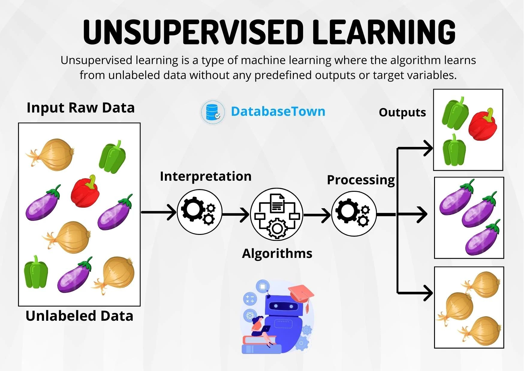
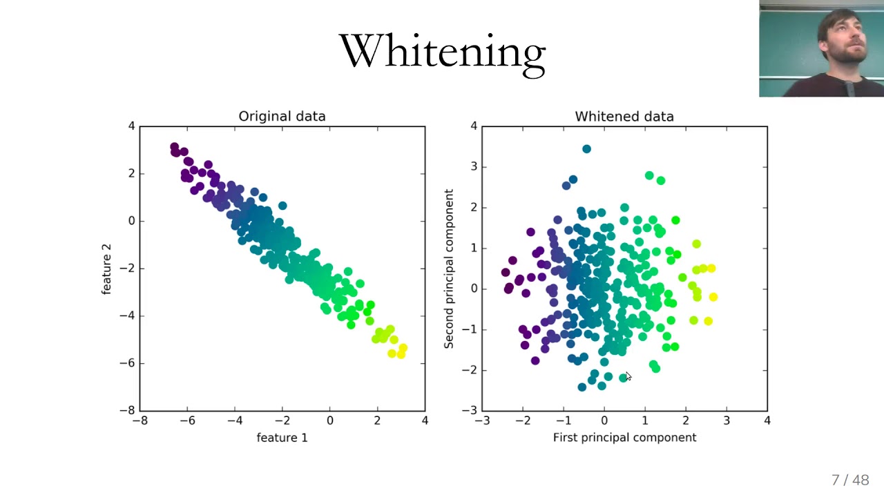
Principal Component Analysis (PCA): PCA is a widely used unsupervised dimensionality reduction technique. It identifies a new set of orthogonal variables called principal components that capture the maximum variance in the data. By projecting the data onto a lower-dimensional subspace defined by these principal components, PCA reduces the dimensionality while retaining most of the important information.
Linear Discriminant Analysis (LDA): LDA is a supervised dimensionality reduction technique that aims to find a subspace that maximizes class separability. It considers the class labels of the data points to identify the directions that best discriminate between different classes. LDA is commonly used for classification tasks where the goal is to reduce the dimensionality while preserving class information.
t-SNE (t-Distributed Stochastic Neighbor Embedding): t-SNE is a nonlinear dimensionality reduction technique that is particularly effective in visualizing high-dimensional data. It focuses on preserving local similarities in the data by mapping each data point to a lower-dimensional space. t-SNE is often used for exploratory data analysis and clustering tasks.
Autoencoders: Autoencoders are neural network models that are trained to reconstruct the input data from a lower-dimensional latent space. By constraining the network to have a bottleneck layer with fewer units, autoencoders can learn a compressed representation of the data. Autoencoders can be used for both unsupervised and semi-supervised dimensionality reduction tasks.

These are just a few examples of the many dimensionality reduction techniques available. The choice of technique depends on the specific characteristics of the data, the goals of analysis, and the requirements of the machine learning task at hand.

It is important to note that dimensionality reduction is not a one-size-fits-all solution, and it is essential to carefully evaluate the results and consider the trade-offs between dimensionality reduction and the specific application requirements.

Principal Component Analysis (PCA)

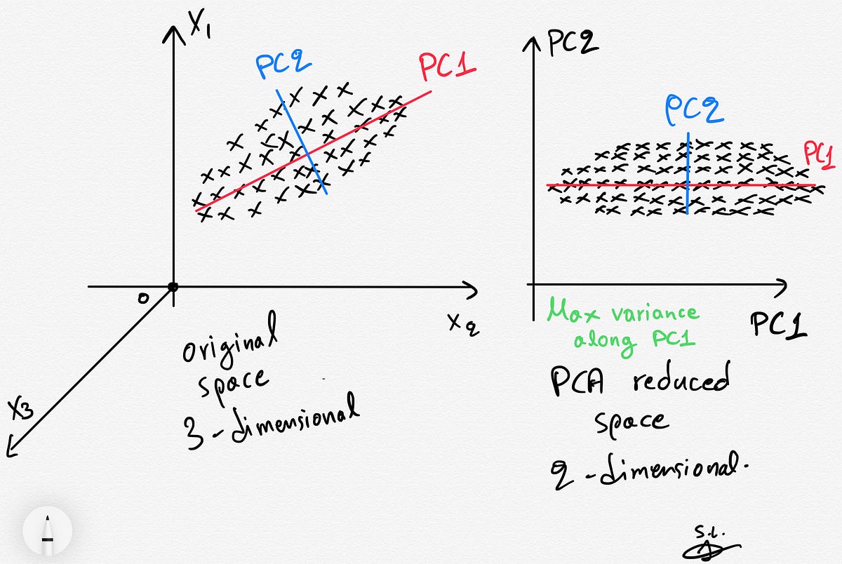
Principal Component Analysis (PCA) is a widely used dimensionality reduction technique that aims to transform high-dimensional data into a lower-dimensional space while preserving the maximum amount of information. It achieves this by identifying a new set of uncorrelated variables called principal components that capture the most significant variation in the data.

The key idea behind PCA is to find a subset of the original features, known as principal components, that explain the majority of the variance in the data. These principal components are ordered, with the first component explaining the most variance, followed by the second component, and so on. By selecting the top principal components, we can effectively reduce the dimensionality of the dataset while retaining as much relevant information as possible.

The process of performing PCA involves several steps. First, the data is standardized to have zero mean and unit variance to ensure that all variables are on the same scale. Next, the covariance matrix or the correlation matrix of the standardized data is computed. This matrix provides information about the linear relationships between the variables.

PCA then decomposes the covariance matrix into its eigenvectors and eigenvalues. The eigenvectors represent the directions in the original feature space, and the eigenvalues indicate the importance of these directions. The eigenvectors with the highest eigenvalues correspond to the principal components, explaining the most variance in the data.

Once the eigenvectors and eigenvalues are computed, the principal components can be obtained by projecting the data onto these vectors. The number of principal components selected determines the dimensionality of the reduced space.

PCA has several benefits. Firstly, it reduces the dimensionality of the data, making it easier to visualize and analyze. It also helps in removing noise and redundant features, leading to improved computational efficiency and model performance. Additionally, PCA can uncover hidden patterns and provide insights into the underlying structure of the data.

However, it is important to note that PCA assumes linearity and may not perform well on datasets with nonlinear relationships. It is also sensitive to outliers and can be influenced by the scaling of the variables. Moreover, the interpretability of the reduced features may be challenging as they are combinations of the original variables.

In summary, Principal Component Analysis (PCA) is a powerful technique for dimensionality reduction that can be applied to a wide range of datasets. By identifying the orthogonal directions that capture the most variation in the data, PCA allows for the creation of a lower-dimensional representation that retains the essential information for analysis and modeling.

Linear Discriminant Analysis (LDA)

Linear Discriminant Analysis (LDA) is a dimensionality reduction technique that focuses on finding a lower-dimensional subspace that maximizes the separation between classes in a supervised learning setting. Unlike PCA, which is an unsupervised technique, LDA takes into account the class labels of the data points to guide the reduction process.

The main objective of LDA is to find a set of linear combinations of the original features, known as discriminant functions, that maximize the between-class scatter while minimizing the within-class scatter. This means that LDA seeks to project the data onto a lower-dimensional space where the different classes are well-separated.

To achieve this, LDA computes the scatter matrices of the data. The within-class scatter matrix represents the spread of the data points within each class, while the between-class scatter matrix measures the separation between class means. The goal is to maximize the ratio of the between-class scatter to the within-class scatter.

By finding the eigenvectors and eigenvalues of the generalized eigenvalue problem defined by the scatter matrices, LDA determines the discriminant functions, which form the basis of the lower-dimensional subspace. The number of discriminant functions selected specifies the dimensionality of the reduced space.

LDA has several applications, particularly in classification tasks. By reducing the dimensionality of the data while preserving class information, LDA helps improve the efficiency and accuracy of classification algorithms. It can also aid in visualizing the data by projecting it onto a lower-dimensional space.

However, it is important to consider a few limitations of LDA. Firstly, LDA assumes that the data follows a Gaussian distribution and that the classes have equal covariance matrices. If these assumptions are violated, the performance of LDA may be affected. Additionally, LDA is a linear technique and may not capture nonlinear relationships in the data. In such cases, nonlinear dimensionality reduction techniques such as kernel PCA or t-SNE may be more appropriate.

In summary, Linear Discriminant Analysis (LDA) is a powerful dimensionality reduction technique that considers class labels to reduce the dimensionality of the data while preserving class separation. By maximizing between-class scatter and minimizing within-class scatter, LDA helps in enhancing classification performance and visualizing the data in lower-dimensional spaces.

t-SNE (t-Distributed Stochastic Neighbor Embedding)

t-SNE (t-Distributed Stochastic Neighbor Embedding) is a nonlinear dimensionality reduction technique that is particularly effective in visualizing high-dimensional data. It aims to reveal the underlying structure and patterns by mapping the data points to a lower-dimensional space in a way that preserves local similarities.

The key idea behind t-SNE is to model similarities between data points in the high-dimensional space and map them to similarities in the low-dimensional space. Unlike linear techniques such as PCA, t-SNE does not make any assumptions about the data distribution and can capture complex nonlinear relationships.

t-SNE builds a probability distribution over pairs of high-dimensional data points, measuring the similarity between them. This probability distribution is then compared to a similar probability distribution in the low-dimensional space. The goal is to minimize the divergence between these two distributions, ensuring that similar data points in the original space are still close in the reduced space.

The optimization process in t-SNE involves minimizing the Kullback-Leibler divergence between the two distributions using stochastic gradient descent. By iteratively updating the positions of the data points in the high-dimensional and low-dimensional spaces, t-SNE gradually converges to a solution that represents the data in a lower-dimensional form while preserving local structures and relationships.

t-SNE is commonly used for data visualization purposes, as it can effectively uncover clusters, patterns, and outliers in high-dimensional datasets. It has been applied to various fields, including biology, computer vision, and natural language processing.

While t-SNE provides valuable visualizations, it is important to note that it may not preserve global structure as well as it does local structure. This means that distances between data points in the low-dimensional space may not accurately reflect their true distances in the high-dimensional space. Therefore, caution should be exercised when interpreting the distances and scales in t-SNE plots.

Additionally, t-SNE can be sensitive to the choice of parameters, such as the perplexity hyperparameter, which controls the balance between local and global aspects of the data. Iterative runs with different parameter settings may be necessary to obtain the most meaningful visual representation of the data.

In summary, t-SNE is a powerful nonlinear dimensionality reduction technique that excels at visualizing high-dimensional data. By preserving local similarities and capturing intricate patterns, t-SNE provides insights into the underlying structure of the data, making it a valuable tool for exploratory data analysis and clustering tasks.

Autoencoders

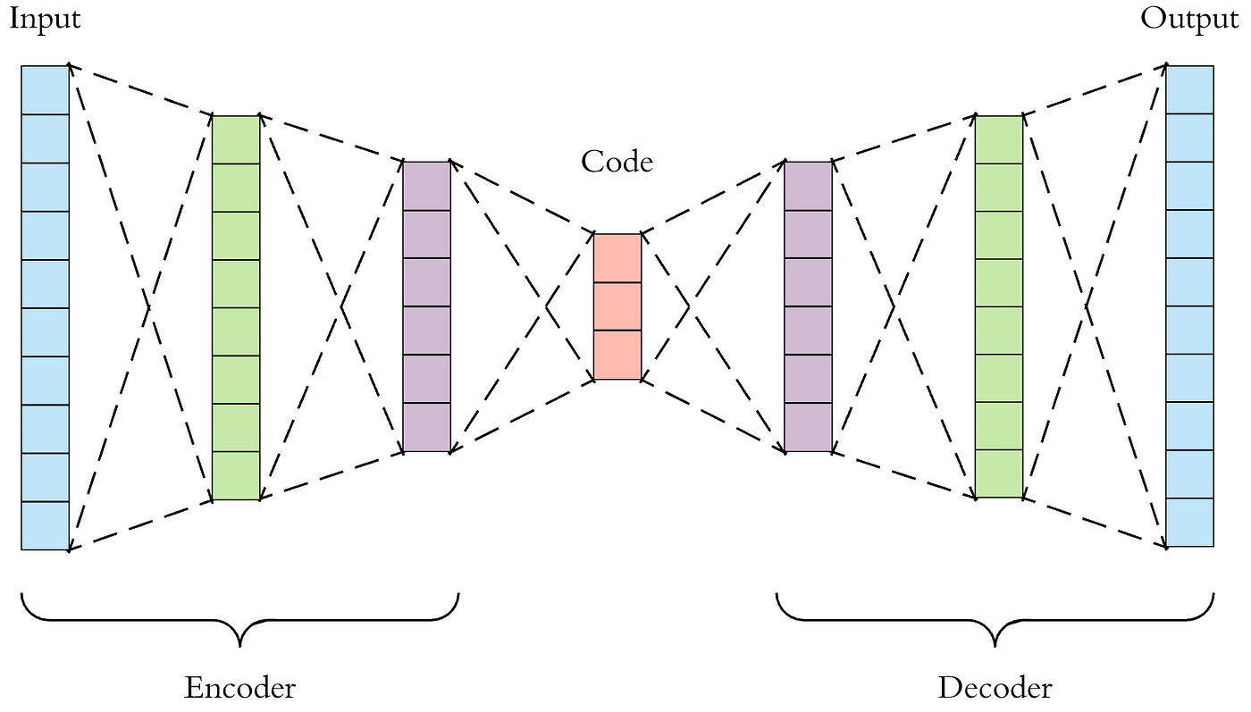
Autoencoders are neural network models used for unsupervised dimensionality reduction. They are capable of learning a compressed representation of the input data, known as the latent space, by training the network to reconstruct the original input from this lower-dimensional space.

The architecture of an autoencoder typically consists of an encoder and a decoder. The encoder takes the input data and maps it to a lower-dimensional representation, compressing the data into a bottleneck layer. The decoder then reconstructs the original input from this compressed representation.

The objective of training an autoencoder is to minimize the difference between the input and the reconstructed output. Through the backpropagation algorithm, the network adjusts its parameters to minimize the reconstruction error, encouraging the network to capture the most important features of the data in the latent space.

Autoencoders have several advantages in dimensionality reduction. They can capture complex patterns and nonlinear relationships in the data, making them suitable for a wide range of applications. Compared to other techniques, autoencoders can learn hierarchical representations, allowing for more precise and expressive encoding of the data.

Furthermore, autoencoders can handle missing or noisy data by learning to reconstruct the original input from corrupted or incomplete samples. This ability makes them robust to data imperfections and useful in scenarios where data quality is a concern.

Autoencoders have various use cases, including anomaly detection, data denoising, and feature extraction. They can also be utilized in semi-supervised learning, where labeled data is scarce, as the learned representation in the latent space can help in improving classification performance.

However, it is essential to consider the limitations of autoencoders. They can be sensitive to the choice of network architecture and hyperparameters, and their performance heavily depends on the quality and representativeness of the training data. Autoencoders might struggle with datasets that have a high degree of irregularity or when the dimensions have different scales.

In summary, autoencoders are powerful neural network models capable of learning compressed representations of data in an unsupervised manner. They can handle complex patterns and noisy data, making them valuable for dimensionality reduction, anomaly detection, and feature extraction tasks.

Benefits and Limitations of Dimensionality Reduction

Dimensionality reduction techniques offer several benefits in data analysis and machine learning. However, it is important to be aware of their limitations. Let’s explore the benefits and limitations of dimensionality reduction:

Benefits:

Improved computational efficiency: By reducing the number of features, dimensionality reduction techniques decrease the computational complexity of data analysis and machine learning algorithms. This leads to faster training and inference times, allowing for more efficient model development and deployment.
Enhanced model performance: Dimensionality reduction removes noise and irrelevant features, leading to improved model accuracy. By focusing on the most informative features, dimensionality reduction techniques help the models capture the underlying patterns in the data more effectively.
Overcoming the curse of dimensionality: High-dimensional data presents challenges due to the vast amount of data required for reliable analysis and modeling. Dimensionality reduction mitigates the curse of dimensionality by reducing the dimensionality of the data, making it more manageable and easier to work with.
Data visualization: The reduced-dimensional representation of the data obtained through dimensionality reduction techniques aids in data visualization. It allows for effective plotting and interpretation of the data, enabling the identification of previously unseen patterns and relationships.
Improved interpretability: High-dimensional datasets can be difficult to interpret. By reducing the dimensionality, the data becomes more concise and interpretable. This enables researchers, analysts, and stakeholders to understand and explain the factors influencing a particular outcome, leading to better decision-making.

Limitations:

Information loss: Dimensionality reduction inevitably involves some loss of information. While efforts are made to retain the most relevant information, reducing the number of features can result in the loss of intricate details or subtle nuances present in the original high-dimensional data.
Choice of technique: There is no one-size-fits-all dimensionality reduction technique. Different techniques have different assumptions and may perform differently depending on the dataset and application. It is crucial to select the most appropriate technique based on the specific characteristics and requirements of the data.
Assumption violations: Some dimensionality reduction techniques make assumptions about the data, such as linearity or specific distributional properties. If these assumptions are violated, the performance of the technique may be compromised, and alternative methods might be necessary.
Computational complexity: Although dimensionality reduction can improve computational efficiency in some cases, certain techniques, such as t-SNE or highly nonlinear methods, can be computationally intensive and may require substantial computational resources.
Interpretability challenges: While dimensionality reduction can enhance interpretability to some extent, the reduced features are often combinations of the original variables, making it challenging to interpret them directly. Additional efforts may be required to establish the meaning and significance of the reduced features.

In summary, dimensionality reduction offers various benefits, including improved computational efficiency, enhanced model performance, and better interpretability. However, it is crucial to consider the limitations, such as information loss, choice of technique, assumption violations, and interpretability challenges, when applying dimensionality reduction techniques to real-world datasets.

Conclusion

Dimensionality reduction is a vital technique in machine learning that addresses the challenges posed by high-dimensional data. It allows for the transformation of complex datasets into lower-dimensional representations, providing benefits such as improved computational efficiency, enhanced model performance, and better interpretability.

Throughout this article, we have explored various dimensionality reduction techniques. Principal Component Analysis (PCA) is a popular unsupervised technique that identifies the directions of maximum variance in the data. Linear Discriminant Analysis (LDA), on the other hand, is a supervised technique that aims to find a subspace that maximizes class separability. t-SNE is known for its ability to effectively visualize high-dimensional data by preserving local relationships. Autoencoders, a type of neural network model, learn a compressed representation of the input data through an unsupervised approach.

While dimensionality reduction techniques offer numerous benefits, including improved computational efficiency, enhanced model performance, and better interpretability, they also have limitations. Information loss is inevitable in dimensionality reduction, and the choice of technique, assumption violations, and interpretability challenges should be carefully considered.

It is important to select the most appropriate dimensionality reduction technique based on the specific characteristics of the data and the goals of the analysis. Additionally, it is crucial to evaluate the results and consider the trade-offs between dimensionality reduction and the specific requirements of the machine learning task.

Dimensionality reduction is a powerful tool that can uncover hidden patterns, simplify complex data, and facilitate the analysis and interpretation of high-dimensional datasets. By effectively reducing the dimensionality of the data, we can gain valuable insights, improve computational efficiency, and enhance the overall performance of machine learning models.