What Does PCA Do In Machine Learning

Introduction

Welcome to the fascinating world of machine learning! In this rapidly evolving field, one of the key challenges is dealing with high-dimensional data. As datasets grow larger and more complex, it becomes increasingly difficult to extract meaningful insights and patterns.

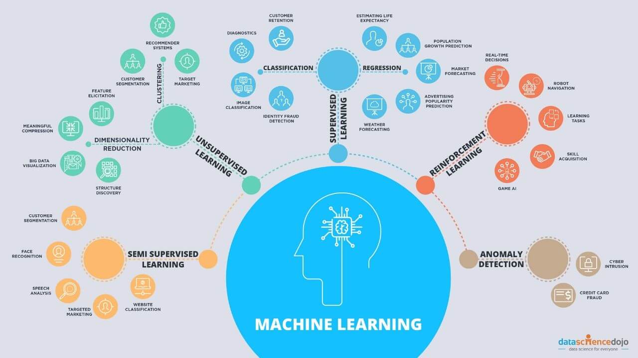
This is where Principal Component Analysis (PCA) comes into play. PCA is a dimensionality reduction technique widely used in machine learning and data analysis to simplify the feature space and improve computational efficiency. By transforming high-dimensional data into a lower-dimensional representation, PCA allows for easier interpretation and visualization of the data.

But what exactly is PCA and how does it work? In this article, we will explore the basics of PCA and its role in machine learning. We will also discuss the benefits and limitations of using PCA as well as its application in various domains.

So, if you’re ready to delve into the world of PCA and discover its power in simplifying complex data, let’s get started!

What is PCA?

Principal Component Analysis (PCA) is a statistical technique used to reduce the dimensionality of a dataset while retaining as much information as possible. It analyzes the correlation between variables and identifies a smaller set of uncorrelated variables, known as principal components, that capture the most significant variation in the data.

The basic idea behind PCA is to transform a dataset consisting of a large number of variables into a smaller set of orthogonal variables. Orthogonal variables are independent of each other and are ordered by the amount of variance they explain in the original data.

Each principal component is a linear combination of the original variables, where the coefficients of this combination are obtained using an eigenvector decomposition of the covariance matrix. These coefficients, called loadings, indicate the contribution of each original variable to the principal component.

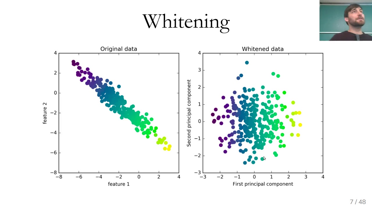
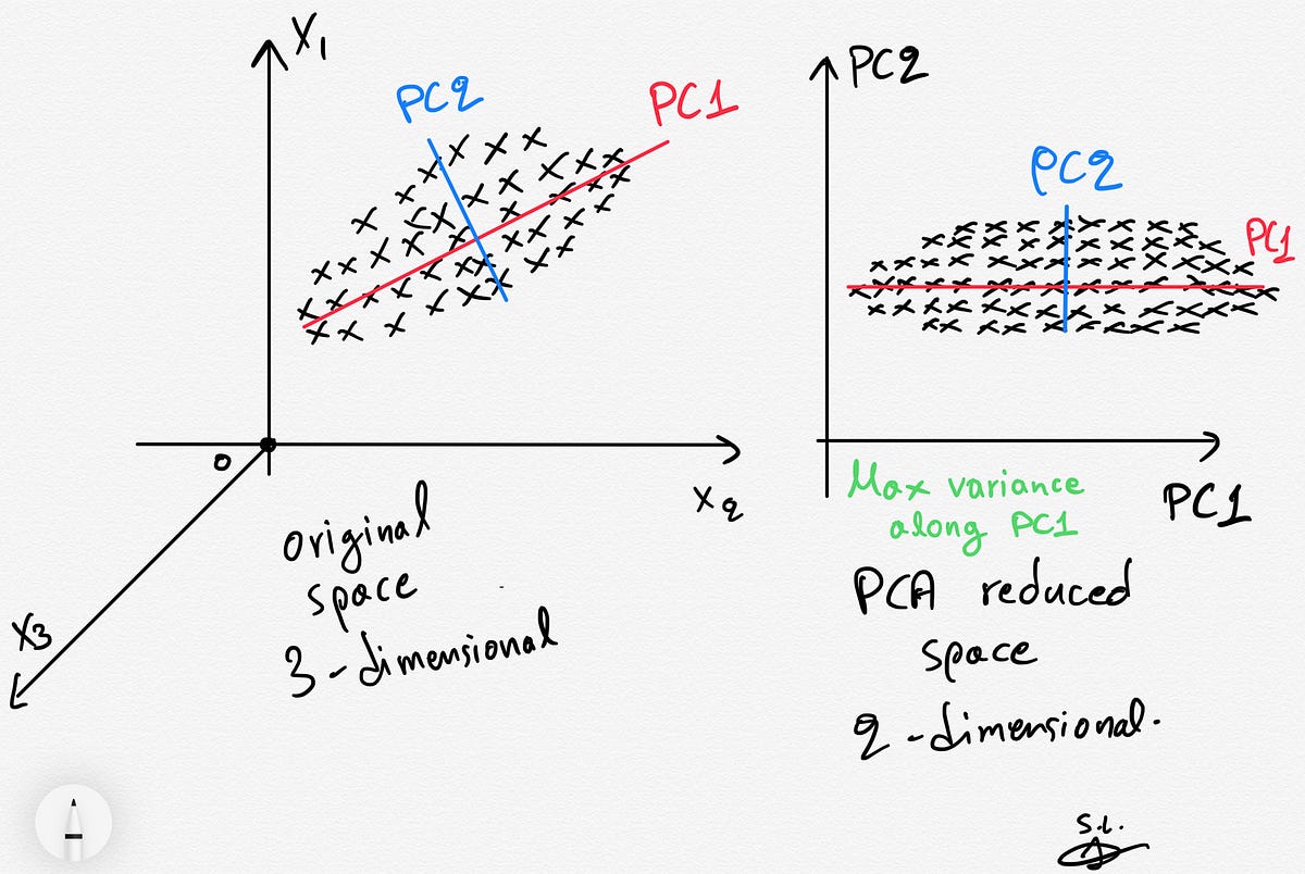
PCA can be thought of as a rotation of the coordinate system in the feature space, aligning the axes with the directions of maximum variance. The first principal component represents the direction in the feature space along which the data varies the most, while the subsequent components capture the remaining variance in decreasing order.

This reduction in dimensionality is particularly valuable when dealing with high-dimensional data, as it allows us to focus on the most relevant information and discard noise or redundant variables. By identifying the principal components that capture the majority of the variance, PCA simplifies the data and facilitates subsequent analysis, data visualization, and modeling.

How PCA works

PCA is a mathematical algorithm that systematically transforms a high-dimensional dataset into a lower-dimensional representation. The key steps involved in PCA can be summarized as follows:

1. Standardize the data: Before applying PCA, it is important to standardize the data by rescaling each variable to have zero mean and unit variance. This step ensures that all variables are on a similar scale, preventing any undue influence on the PCA results.
2. Compute the covariance matrix: The next step is to calculate the covariance matrix, which describes the relationships between pairs of variables in the dataset. The covariance measures how changes in one variable are related to changes in another. The diagonal elements of the covariance matrix represent the variance of each variable, while the off-diagonal elements represent the covariances between variables.
3. Compute the eigenvalues and eigenvectors: Using the covariance matrix, we can find the eigenvalues and eigenvectors. The eigenvalues represent the amount of variance explained by each principal component, while the corresponding eigenvectors indicate the direction in which the data varies the most.
4. Select the desired number of principal components: Depending on the goals of the analysis, we need to decide how many principal components to retain. This can be based on a predetermined threshold of explained variance or by examining a scree plot, which displays the eigenvalues in descending order.
5. Compute the principal components: Once the desired number of principal components is determined, we can compute the principal components by projecting the standardized data onto the eigenvectors. This transformation yields a new dataset with a reduced number of variables.

The result of PCA is a set of principal components, where the first component explains the maximum amount of variance in the dataset, the second component explains the next highest variance, and so on. These components are orthogonal to each other, meaning they are uncorrelated.

By selecting a smaller number of principal components, we can effectively reduce the dimensionality of the dataset while capturing the majority of its variability. This allows for easier interpretation and visualization of the data, as well as more efficient computational analysis in subsequent stages of machine learning or data exploration.

Selecting the Number of Principal Components

One important consideration in PCA is determining the appropriate number of principal components to retain. This decision is crucial as it directly affects the amount of variance captured by the reduced-dimension representation of the data.

There are several methods to help determine the optimal number of principal components:

1. Explained Variance: This method involves examining the cumulative explained variance plot. The plot shows the cumulative proportion of variance explained by each principal component. We can set a threshold, such as 80% or 90% explained variance, and select the number of principal components that surpass this threshold. This ensures that a substantial amount of information is retained while reducing the dimensionality of the data.
2. Scree Plot: The scree plot displays the eigenvalues of the principal components in descending order. The eigenvalues indicate the amount of variance explained by each component. We can visually inspect the scree plot and select the number of components at the point where the eigenvalues show a significant drop-off. This can be subjective, but it provides a graphical representation of the diminishing returns of adding more principal components.
3. Cumulative Variance: Similar to the explained variance method, the cumulative variance approach involves selecting the number of principal components where the cumulative proportion of variance reaches a desirable threshold. This method provides a more comprehensive view of how much information is captured as we incrementally include more principal components.
4. Domain Knowledge: In some cases, domain knowledge or prior research can guide the selection of the number of principal components. For example, if there are specific variables or features that are known to be more important or influential in the domain, they can be given priority in the PCA analysis.

It’s important to keep in mind that the selected number of principal components should strike a balance between retaining enough information and reducing dimensionality. Retaining too few principal components may result in a loss of important information, while retaining too many may not provide significant additional insights or improvements in computational efficiency.

Ultimately, the choice of the number of principal components depends on the specific dataset, the goals of the analysis, and the trade-offs between information retention and computational complexity.

Applying PCA in Machine Learning

PCA has various applications in machine learning, where it can help improve the performance and efficiency of models by reducing the dimensionality of the input data. Here are some common use cases of applying PCA in machine learning:

1. Feature Extraction: PCA can be used to extract the most important features from a high-dimensional dataset. By selecting a subset of the principal components that capture the majority of the variance, we can create a lower-dimensional representation of the data that still retains the most crucial information. This feature extraction step can be beneficial when working with large datasets or when dealing with computational limitations.
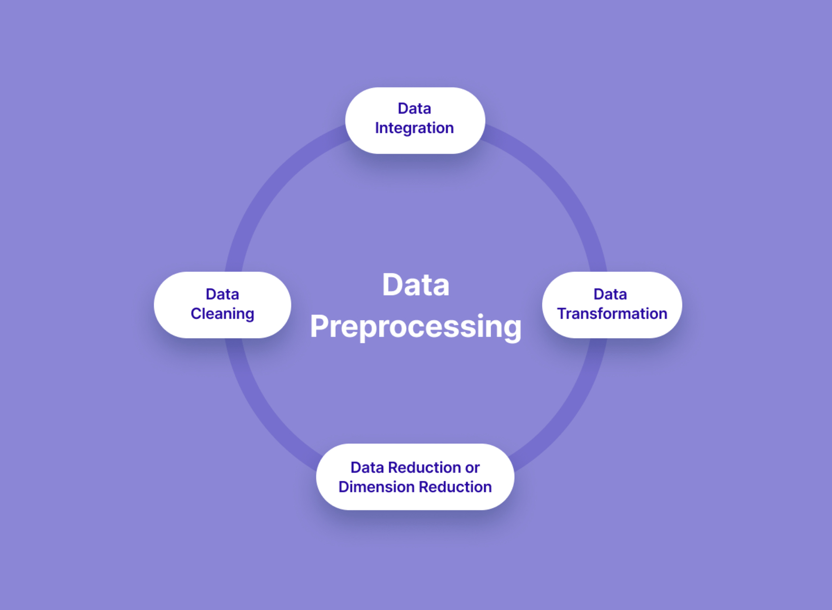
2. Data Preprocessing: PCA can also be used as a preprocessing step to remove noise or redundant information from the dataset. By eliminating low-variance components, we can reduce the impact of noisy or irrelevant variables on the learning process. This helps improve the robustness and generalization of machine learning models, especially in scenarios where the dataset contains a large number of noisy or irrelevant features.
3. Visualization: One of the key advantages of PCA is its ability to create lower-dimensional representations of the data that can be easily visualized. By reducing the dimensions, we can plot the data points on a 2D or 3D graph, making it easier to explore and interpret the relationships between variables. This visualization can aid in identifying clusters, patterns, or outliers in the data, leading to valuable insights and guiding further analysis.
4. Model Training: PCA can be used to speed up the training process of machine learning models, especially in cases where the original dataset is too large or when dealing with a high number of features that may lead to overfitting. By reducing the dimensionality of the data, the computational complexity of the learning algorithm can be significantly reduced without sacrificing much information. This acceleration in training time can be crucial in practical scenarios where time is a critical factor.

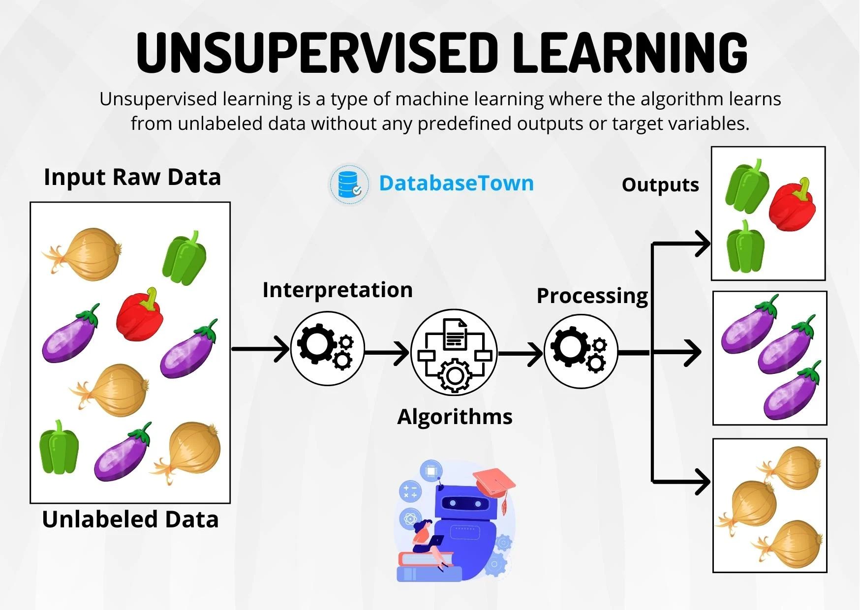
It’s important to note that PCA is typically applied in unsupervised learning scenarios or as a preprocessing step before supervised learning. It helps in understanding the underlying structure of the data and simplifying it while preserving the essential information. However, depending on the nature of the problem and the specific dataset, it’s crucial to evaluate the impact of using PCA on the final performance of the machine learning model as sometimes there might be a trade-off between dimensionality reduction and model accuracy.

Benefits of Using PCA

Principal Component Analysis (PCA) offers several benefits when applied in machine learning and data analysis. Here are some of the key advantages of using PCA:

1. Dimensionality Reduction: One of the main advantages of PCA is its ability to reduce the dimensionality of high-dimensional datasets. By transforming the data into a lower-dimensional space, PCA simplifies the analysis and alleviates the “curse of dimensionality”. This reduction in dimensionality improves computational efficiency, reduces storage requirements, and facilitates visualization and interpretation of the data.
2. Noise and Redundancy Removal: PCA can effectively remove noise and redundant information from the dataset. By identifying the principal components that capture the majority of the variation in the data, PCA eliminates the influence of variables with low variances, which are often associated with noise. It also identifies and eliminates redundant features, helping to improve the robustness and generalization of machine learning models.
3. Data Visualization: PCA provides a powerful tool for data visualization. By transforming high-dimensional data into a lower-dimensional space, it becomes easier to visualize and explore the relationships between variables. This can lead to valuable insights and facilitate decision-making processes. Visualizing the data using PCA can reveal clusters, patterns, or outliers that may not be apparent in the original high-dimensional space.
4. Computational Efficiency: With its dimensionality reduction capabilities, PCA can significantly improve the computational efficiency of machine learning algorithms. By reducing the number of features, the training and inference time of models can be substantially reduced. This accelerated performance is particularly beneficial in scenarios where time is a critical factor, such as real-time applications or large-scale datasets.
5. Improved Model Performance: While PCA itself does not directly improve model performance, it can indirectly enhance the performance by reducing overfitting. By removing noise and uninformative features, PCA helps to prevent models from being overly sensitive to irrelevant variations in the data. This regularization effect can improve the model’s generalization ability, leading to better performance on unseen data.

Overall, PCA is a valuable tool in the machine learning and data analysis toolkit. It enables dimensionality reduction, noise and redundancy removal, data visualization, and improved computational efficiency, all of which contribute to more efficient and effective data analysis and modeling.

Limitations of PCA

While Principal Component Analysis (PCA) offers numerous benefits, it is important to be aware of its limitations and potential drawbacks. Here are some of the key limitations to consider when using PCA:

1. Linearity Assumption: PCA assumes that the underlying data relationships are linear. If the relationships are non-linear, PCA may not accurately capture the true structure of the data. In such cases, non-linear dimensionality reduction techniques such as Kernel PCA may be more suitable.
2. Loss of Interpretability: Although PCA simplifies the data by reducing dimensionality, it may come at the cost of interpretability. The principal components obtained through PCA are linear combinations of the original variables and may not have direct physical or intuitive meaning. While PCA provides a useful representation for computational purposes, understanding the specific contribution of each original variable to the principal components can be challenging.
3. Information Loss: The dimensionality reduction in PCA comes at the expense of information loss. By selecting a smaller number of principal components, some amount of information in the dataset is inevitably discarded. The challenge lies in finding a balance between reducing dimensionality and maintaining an acceptable level of information retention for the specific application.
4. Impact of Outliers: PCA can be sensitive to outliers in the dataset. Outliers can have a significant influence on the covariance matrix and, consequently, on the principal components. It is important to handle outliers appropriately or consider using robust variants of PCA to minimize their impact.
5. Scaling Sensitivity: PCA is sensitive to the scaling of variables. It is crucial to standardize the data before applying PCA to ensure that variables with larger variances do not dominate the results. Failing to properly scale the data can lead to misleading results and inaccurate interpretations.
6. Curse of Dimensionality: Although PCA addresses the issue of high dimensionality, it does not fully eliminate the problems associated with the curse of dimensionality. In some cases, even after reducing dimensionality, the remaining number of principal components may still be too high, leading to computational challenges and potential overfitting.

Understanding these limitations can help in making informed decisions when applying PCA. It is important to carefully assess the specific characteristics of the data and the goals of the analysis to determine if PCA is the appropriate technique or if there are alternative methods that may better suit the requirements.

Conclusion

Principal Component Analysis (PCA) is a powerful technique that allows for the reduction of dimensionality in datasets, bringing numerous benefits to machine learning and data analysis. By transforming high-dimensional data into a lower-dimensional representation, PCA simplifies analysis, improves computational efficiency, and enhances data visualization.

We started by understanding the fundamentals of PCA, including its purpose in simplifying the feature space and capturing the most significant variation in the data. We explored how PCA works by computing the covariance matrix, calculating eigenvalues and eigenvectors, and selecting the desired number of principal components.

Throughout this article, we have seen the practical applications of PCA in machine learning. It can be used for feature extraction, data preprocessing, visualization, and improving model performance. PCA effectively reduces the dimensionality of the data, removes noise and redundancy, accelerates training time, and facilitates the exploration of relationships between variables.

However, we have also discussed the limitations of PCA. It assumes linearity, may sacrifice interpretability, involves information loss, can be sensitive to outliers, requires appropriate scaling, and may not fully overcome the challenges of the curse of dimensionality. Being aware of these limitations helps in understanding when and how to properly utilize PCA.

In conclusion, Principal Component Analysis is a valuable tool that empowers data scientists and machine learning practitioners to address the challenges posed by high-dimensional data. Understanding its principles, applications, and limitations allows for informed decision-making and effective utilization of PCA in various domains.