Introduction
Data preprocessing is an essential step in machine learning that involves preparing raw data for analysis. It is a crucial part of the data pipeline as it lays the foundation for building accurate and reliable machine learning models. In simple terms, data preprocessing refers to the transformation of raw data into a format that is suitable for further analysis by machine learning algorithms.
Raw data is typically unstructured, contains inconsistencies, missing values, and outliers, making it difficult for machine learning algorithms to process effectively. Data preprocessing helps in addressing these issues by cleaning, transforming, and organizing the data in a way that makes it easier to work with.
With the ever-increasing availability of vast amounts of data, data preprocessing has become more important than ever. It is crucial to ensure that the data is of high quality, reliable, and ready for analysis. By performing thorough data preprocessing, we can minimize the risk of errors or biases in the machine learning models, improve the accuracy of predictions, and extract meaningful insights from the data.
Data preprocessing involves various techniques and steps, such as handling missing data, dealing with categorical variables, performing feature scaling, and handling outliers and noisy data. Each of these steps plays a vital role in transforming the raw data into a usable form that can be fed into machine learning algorithms.
In this article, we will dive deeper into the importance of data preprocessing in machine learning and explore the key steps involved in the data preprocessing pipeline. By understanding the impact of data preprocessing and mastering the techniques involved, data scientists and machine learning practitioners can greatly enhance the performance and accuracy of their models.
What is Data Preprocessing
Data preprocessing is the process of transforming raw data into a clean, consistent, and structured form that can be analyzed and utilized by machine learning algorithms. It involves a series of techniques and steps aimed at cleaning and preparing the data for further analysis.
The raw data collected for machine learning tasks is often riddled with inconsistencies, missing values, outliers, and various other issues. Data preprocessing helps in addressing these challenges and ensures that the data is in a suitable format for machine learning models to process effectively.
One of the primary goals of data preprocessing is to clean the data by removing any inconsistencies or errors. This may involve handling missing data, correcting erroneous entries, and eliminating duplicate records. Cleaning the data ensures that the machine learning models are not biased or influenced by incorrect or incomplete information.
Furthermore, data preprocessing aims to transform the data into a consistent format that can be easily interpreted by machine learning algorithms. This includes converting categorical variables into numerical representations, standardizing data ranges, and normalizing the data to eliminate any scale or unit discrepancies.
Data preprocessing also involves handling outliers and noisy data points. Outliers are data points that deviate significantly from the rest of the dataset and can have a significant impact on model performance. By understanding the nature of the data and the underlying domain, outliers can be identified and appropriately dealt with. Similarly, noisy data, which contains random or irrelevant information, can be filtered out or smoothed to improve the quality of the data.
Another aspect of data preprocessing is feature scaling, which involves bringing different features to a similar scale to avoid bias towards certain variables. This is particularly important for distance-based algorithms, where features with larger ranges can overshadow those with smaller ranges. Feature scaling ensures that all variables contribute equally to the model’s decision-making process.
Overall, data preprocessing is a critical step in the machine learning pipeline. It helps in transforming raw data into a format that is suitable for analysis and enhances the accuracy and reliability of machine learning models. By effectively preprocessing the data, practitioners can lay the foundation for building robust models that can extract valuable insights and make accurate predictions.
Why is Data Preprocessing important in Machine Learning
Data preprocessing plays a crucial role in machine learning and is considered a fundamental step in building accurate and reliable models. There are several reasons why data preprocessing is important in the machine learning process.
Firstly, data preprocessing helps in improving the quality of the data. Raw data often contains inconsistencies, errors, and missing values, which can negatively impact model performance. By addressing these issues through data preprocessing techniques, such as handling missing data and cleaning the dataset, we can ensure that the data is reliable and of high quality.
In addition, data preprocessing helps in handling categorical variables. Machine learning algorithms typically operate on numerical data, and categorical variables need to be encoded into a numerical format. By applying techniques like one-hot encoding or label encoding, we can convert categorical variables into numerical representations, allowing the algorithms to process the data effectively.
Data preprocessing also enables feature scaling, which is crucial for algorithms that are sensitive to the scale of the input features. Scaling the features to a similar range ensures that no specific feature dominates the model’s decision-making process. This leads to more balanced and accurate predictions.
Moreover, data preprocessing helps in handling outliers and noisy data. Outliers, which are data points that deviate significantly from the rest of the dataset, can have a profound impact on model training and prediction. By identifying and appropriately dealing with outliers, we can prevent them from negatively influencing the model’s behavior. Similarly, noisy data, which contains random or irrelevant information, can be filtered out or smoothed to improve the overall quality of the data and enhance model performance.
Data preprocessing also aids in feature extraction, which involves selecting or creating new features that have high predictive power. Through feature extraction techniques like principal component analysis (PCA) or dimensionality reduction algorithms, we can reduce the complexity of the data and focus on the most important features. This not only improves computational efficiency but also helps in avoiding overfitting and improving generalization.
Overall, data preprocessing is essential in machine learning as it helps in improving data quality, handling categorical variables, ensuring feature scaling, dealing with outliers and noisy data, and performing feature extraction. By taking these preprocessing steps, we can create cleaner and more relevant datasets that can significantly enhance model performance and deliver more accurate predictions.
Steps involved in Data Preprocessing
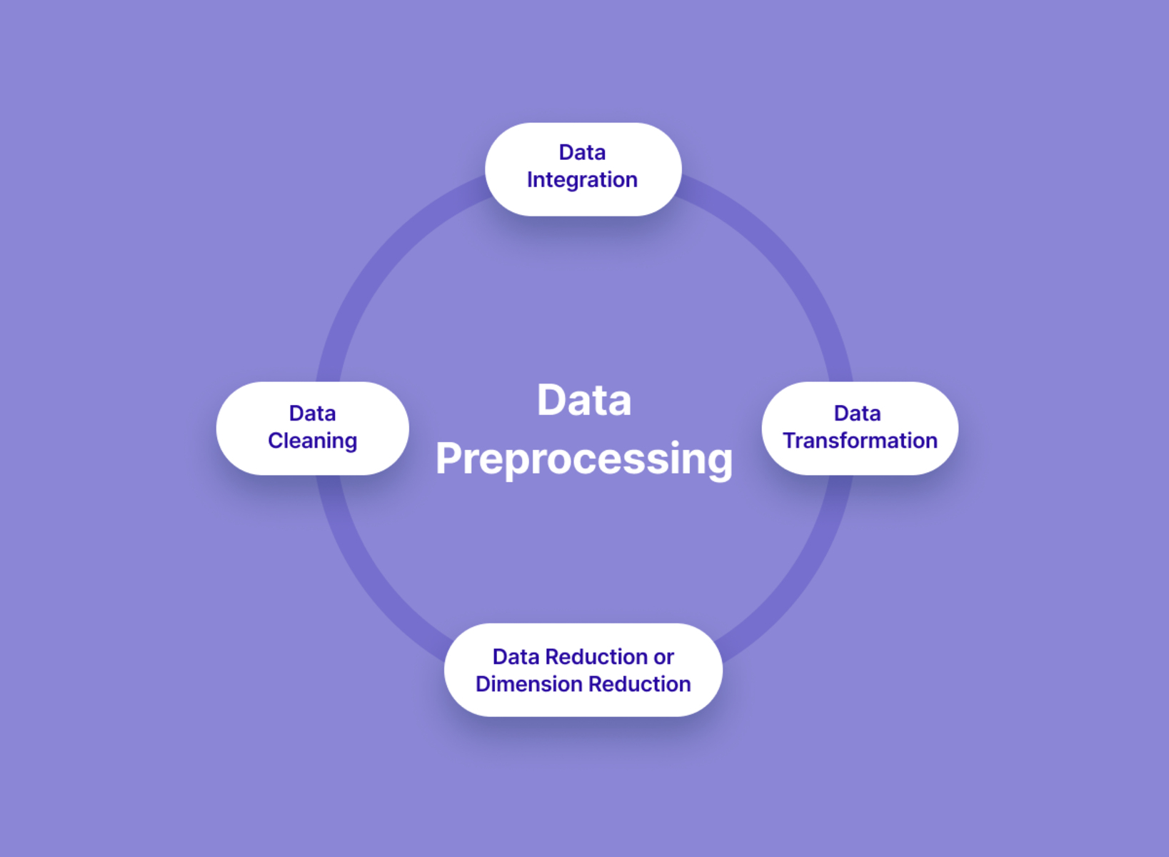
Data preprocessing involves several steps that help to transform raw data into a suitable format for analysis by machine learning algorithms. Let’s explore the key steps involved in the data preprocessing pipeline:
1. Data Cleaning: This step focuses on handling missing data, correcting errors, and dealing with inconsistencies in the dataset. Missing data can be handled by either removing the corresponding records or imputing the missing values based on statistical measures or machine learning techniques.
2. Handling Categorical Data: Machine learning algorithms typically work with numerical data, so it is essential to convert categorical variables into a numerical format. This can be achieved through techniques like one-hot encoding, label encoding, or binary encoding, depending on the nature of the categorical variables.
3. Feature Scaling: Feature scaling ensures that all features are brought to a similar scale to prevent biases and weight imbalances. Common techniques for feature scaling include standardization and normalization. Standardization scales the data to have a mean of 0 and a standard deviation of 1, while normalization scales the data to a specific range, such as between 0 and 1.
4. Handling Outliers: Outliers are data points that deviate significantly from the majority of the data. They can be problematic for machine learning algorithms, affecting model training and prediction accuracy. Outliers can be detected and handled by various statistical methods or using algorithms like the Z-score technique or the Interquartile Range (IQR) method.
5. Handling Noisy Data: Noisy data refers to data that contains random or irrelevant information. It can negatively impact the performance of machine learning models. Noisy data can be filtered out or smoothed using techniques like moving averages or median filtering.
6. Data Encoding: In some cases, data may require encoding to represent categorical or textual information in a meaningful way. Encoding techniques like word embedding or vectorization can be used to convert textual data into numerical representations that can be processed by machine learning algorithms.
7. Feature Extraction: Feature extraction involves reducing the dimensionality of the dataset while preserving its most relevant information. Techniques like Principal Component Analysis (PCA) or Linear Discriminant Analysis (LDA) can be applied to extract the most important features from the dataset.
8. Splitting the Dataset: The final step involves splitting the dataset into training, validation, and testing sets. This allows us to evaluate the model’s performance on unseen data and assess its generalization capabilities.
By following these steps and customizing them based on the specific characteristics and requirements of the dataset, we can preprocess the data effectively, improving the quality, consistency, and suitability for machine learning algorithms.
Handling Missing Data
Missing data is a common issue in datasets and can significantly impact the performance and accuracy of machine learning models. Therefore, handling missing data is an important step in the data preprocessing pipeline. Let’s explore some techniques for handling missing data:
1. Deletion: In this technique, missing data is simply removed from the dataset. If the missing data is relatively small in comparison to the overall dataset, deleting those records may not significantly affect the analysis. However, this method can lead to a loss of valuable information, especially if the missing data is substantial or contains important patterns.
2. Imputation: Imputation is the process of filling in missing values with estimated or imputed values. There are several methods for imputing missing data:
- Mean/Median Imputation: Missing values in numerical variables can be replaced with the mean or median of the available values of that variable. This method provides a simple and commonly used approach but may not work well if the data has outliers or extreme values.
- Mode Imputation: For categorical variables, missing values can be imputed with the mode (most frequent value) of the variable. This method is useful for variables with a limited number of possible values.
- Regression Imputation: Regression models can be used to predict missing values based on other variables in the dataset. A regression model is trained using the available data, and the predicted values are used to impute the missing values. This method can capture the relationships between variables and provide more accurate imputations.
- Multiple Imputation: Multiple imputation involves creating multiple imputed datasets by generating plausible values for the missing data based on statistical methods. This approach takes into account the uncertainty associated with imputing missing values and can provide more reliable results.
3. Advanced Techniques: There are also advanced techniques for handling missing data, such as using machine learning algorithms or time series modeling to impute missing values. These techniques can capture complex relationships in the data and provide more accurate imputations.
It is important to note that the choice of method for handling missing data depends on the nature of the dataset, the amount and patterns of missing data, and the specific requirements of the analysis. It is essential to carefully analyze the dataset and consider the implications of each method before deciding on the most appropriate approach.
Handling missing data effectively can prevent bias, ensure the integrity of the data, and improve the performance of machine learning models. By choosing the right technique for the given dataset, we can mitigate the impact of missing data and ensure that the analysis is based on reliable and complete information.
Handling Categorical Data
Categorical data refers to variables that represent distinct categories or groups, such as gender, color, or product types. Since most machine learning algorithms operate on numerical data, it is essential to convert categorical variables into a numerical format through a process called categorical data encoding. Let’s explore some common techniques for handling categorical data:
1. One-Hot Encoding: One-hot encoding is a technique where each category of a categorical variable is converted into a separate binary feature. For example, if we have a “color” variable with categories red, green, and blue, we can create three binary features: is_red, is_green, and is_blue. Each feature will have a value of 1 if the data point belongs to that category, and 0 otherwise. One-hot encoding helps to avoid assigning artificial numerical weights to categories and allows machine learning models to “understand” the categorical information effectively.
2. Label Encoding: Label encoding involves assigning a numerical label to each category of a categorical variable. Each unique category is assigned a different integer value. For example, if we have a “gender” variable with categories male and female, we can encode them as 0 and 1, respectively. Label encoding is suitable for variables with a natural ordering, where the numerical value itself carries some information. However, for variables without any inherent order, using label encoding may introduce unintended relationships between categories.
3. Ordinal Encoding: Ordinal encoding is a variation of label encoding that takes into account the ordinal relationship between categories. It assigns numerical values to categories based on their order, maintaining the information about the relative ordering of the categories. For example, if we have an “education level” variable with categories high school, bachelor’s degree, and master’s degree, we can encode them as 1, 2, and 3, respectively. Ordinal encoding is suitable when the categories have an inherent order, but it may not be appropriate for variables without a clear ranking.
4. Binary Encoding: Binary encoding combines aspects of one-hot encoding and label encoding by representing each unique category as a binary code. Each category is assigned a unique binary code, and these codes are used to create binary features. Binary encoding reduces the dimensionality compared to one-hot encoding while preserving the categorical information to some extent.
5. Feature Hashing: Feature hashing, also known as the hashing trick, is a technique for handling high-cardinality categorical variables. It involves hashing the categories into a fixed number of features, reducing the dimensionality of the data. Hashing can be a useful technique when the number of unique categories is large, as it helps to avoid the memory and processing constraints associated with one-hot encoding or label encoding.
Choosing the appropriate categorical encoding technique depends on factors such as the nature of the variable, the number of unique categories, and the specific requirements of the machine learning problem. It is important to consider the implications of each technique and the potential impact on model performance.
By converting categorical data into a numerical format, machine learning models can effectively process and analyze the information, leading to improved performance and more accurate predictions.
Feature Scaling
Feature scaling is an important step in data preprocessing that aims to bring different features of a dataset to a similar scale. Scaling the features ensures that no specific feature dominates the learning process of a machine learning algorithm, allowing for a fair comparison and accurate model training. Let’s discuss some common techniques used for feature scaling:
1. Standardization: Standardization, also known as z-score normalization, transforms the data in such a way that it has a mean of 0 and a standard deviation of 1. This is achieved by subtracting the mean value of the feature from each data point and dividing it by the standard deviation. Standardization helps in normalizing the data distribution and is less affected by outliers. It is commonly used when the features exhibit different scales or when the data follows a Gaussian (bell-shaped) distribution.
2. Normalization: Normalization, also known as min-max scaling, scales the data to a specific range, typically between 0 and 1. It calculates the scaled value of each data point by subtracting the minimum value of the feature and dividing it by the difference between the maximum and minimum values. Normalization is useful when the distribution of the data is not Gaussian and when the range of the feature values is known and significant.
3. Robust Scaling: Robust scaling is a technique that is less affected by outliers compared to standardization and normalization. It scales the data using the interquartile range (IQR) instead of the mean and standard deviation. The IQR is calculated by subtracting the 25th percentile from the 75th percentile of the feature values. Robust scaling is useful when the data contains extreme values or when the distribution is non-Gaussian.
4. Log Transformation: In some cases, a log transformation can be used to scale the data. Log transformation compresses the range of values, making it useful when the data has a skewed or exponential distribution. It can help in reducing the impact of extreme values and normalizing the data.
The choice of the appropriate feature scaling technique depends on factors such as the distribution of the data, the presence of outliers, and the requirements of the machine learning algorithm. It is important to note that not all machine learning algorithms require feature scaling. For instance, tree-based algorithms like decision trees and random forests are generally insensitive to the scale of the features.
By applying appropriate feature scaling techniques, we can ensure that all features contribute equally to the model’s decision-making process, prevent biases towards certain variables, and achieve better overall model performance.
Data Normalization
Data normalization, also known as min-max scaling, is a data preprocessing technique that transforms the data to a specific range, typically between 0 and 1. It rescales the feature values so that they fall within a standardized range, making them more comparable and suitable for machine learning algorithms.
The process of data normalization involves calculating the normalized value for each data point by subtracting the minimum value of the feature and dividing it by the difference between the maximum and minimum values. The formula for data normalization can be represented as:
Normalized Value = (x – min) / (max – min)
Normalized data has several benefits in machine learning:
1. Comparable Scale: Normalizing the data brings all features to a similar scale. By doing so, it eliminates the issue of features with larger ranges dominating the learning process. This is particularly important for distance-based algorithms, such as k-nearest neighbors (KNN) or clustering algorithms, where features with larger ranges can overshadow those with smaller ranges.
2. Improved Convergence: Normalization aids in faster convergence during the training of machine learning models. By restricting the feature values to a standardized range, it prevents the learning process from diverging or getting stuck due to large feature values that result in excessively large gradients, affecting the optimization process.
3. Robustness Against Outliers: Normalization is less affected by outliers in the data compared to other scaling techniques. The normalized values are constrained within the range of 0 and 1, reducing the influence of extreme values on the model’s behavior. This helps in reducing the impact of outliers on the overall analysis.
4. Interpretable Data Comparison: Normalized data allows for easier interpretation and comparison between different features. With all features scaled to a similar range, it becomes straightforward to understand the relative importance or contribution of each feature to the model’s predictions.
It is essential to consider the nature of the data and the requirements of the machine learning algorithms before applying data normalization. Not all algorithms require or benefit from normalization. For instance, decision tree-based algorithms and ensemble methods like random forests are generally insensitive to feature scaling.
Data normalization is a vital step in the data preprocessing pipeline that helps in standardizing the range of features, improving convergence, providing robustness against outliers, and enabling interpretable data comparison. By normalizing the data, machine learning models can make fair and accurate predictions while minimizing the biases introduced by varying feature scales.
Data Standardization
Data standardization is a common data preprocessing technique that transforms the data in such a way that it has a mean of 0 and a standard deviation of 1. It is also known as z-score normalization and is particularly useful when the data follows a Gaussian (bell-shaped) distribution.
The process of data standardization involves subtracting the mean of the feature from each data point and dividing it by the standard deviation. This normalizes the data by bringing it to a standardized scale. Mathematically, data standardization can be expressed as:
Standardized Value = (x – mean) / standard deviation
Data standardization provides several benefits in machine learning:
1. Comparable Scale: By standardizing the data, all features are brought to the same scale, making them comparable. This is important for algorithms that are sensitive to the scale of the features, such as support vector machines (SVM) or algorithms that use gradient descent optimization.
2. Improved Convergence: Data standardization aids in faster convergence during the training of machine learning models. It prevents the learning process from being influenced by large feature values that result in excessively large gradients. This helps in optimizing the model’s parameters more efficiently.
3. Robustness Against Outliers: Data standardization is less affected by outliers compared to other scaling techniques. Since it calculates the z-scores based on the mean and standard deviation, outliers have less impact on the resulting standardized values. This makes the analysis more robust and less prone to the influence of extreme values.
4. Preservation of Shape: Standardizing the data does not change the shape or the distribution of the original data. It only rescales the data to have a mean of 0 and a standard deviation of 1. This means that the relative relationships between different data points and the patterns in the data remain unchanged.
It is important to note that not all machine learning algorithms require data standardization. Tree-based algorithms, such as decision trees and random forests, are generally insensitive to feature scaling. However, many linear-based models, such as linear regression or logistic regression, can benefit from data standardization.
Data standardization is a powerful technique in the data preprocessing pipeline that brings features to a comparable scale, improves convergence, provides robustness against outliers, and preserves the shape of the data. By standardizing the data, machine learning models can make fair and accurate predictions while avoiding biases and improper weightings caused by varying feature scales.
Handling Outliers
Outliers are data points that deviate significantly from the rest of the dataset. They can occur due to various reasons, such as measurement errors, data entry mistakes, or rare events. Outliers can have a significant impact on the analysis and performance of machine learning models, making it important to handle them appropriately. Let’s explore some techniques for handling outliers:
1. Detection: Before handling outliers, it is essential to identify them. There are several statistical methods for outlier detection, such as the Z-score method or the Interquartile Range (IQR) method. The Z-score method calculates the standardized value of each data point based on the mean and standard deviation. Data points that have a Z-score above a certain threshold (typically 2 or 3) are considered outliers. The IQR method involves calculating the range between the 25th and 75th percentiles of the data. Data points that fall below the lower range or above the upper range (using a specified threshold, such as 1.5 times the IQR) are considered outliers.
2. Removal: One simple approach to handling outliers is to completely remove them from the dataset. However, removing outliers should be done cautiously, as it can lead to a loss of valuable information. It is typically recommended to remove outliers only when they are clear anomalies and do not represent genuine data points. This should be supported by domain knowledge and clear justification.
3. Transformation: Another approach is to transform the data to reduce the impact of outliers. This can be done through various techniques, such as logarithmic transformation or data smoothing. Logarithmic transformation compresses the extreme values, making the distribution more symmetrical. Data smoothing involves applying techniques, such as moving averages or median filtering, to reduce the noise and fluctuations in the data.
4. Winsorization: Winsorization is a method that replaces extreme values (outliers) with values that are closer to the rest of the data. The extreme values are set to a predetermined percentile value, either on the upper or lower end of the range. This helps in minimizing the impact of outliers without completely removing them.
5. Binning: Binning involves grouping data points into bins and representing each bin with a single representative value. This can help in reducing the impact of individual outliers by aggregating data points into broader categories. Binning should be done based on sound domain knowledge and understanding of the data.
It is important to note that the approach to handle outliers depends on the specific dataset, the nature of the outliers, and the requirements of the analysis. It is crucial to carefully assess the impact of outliers and consider the limitations and implications of each technique before deciding on the most appropriate method.
By appropriately handling outliers, we can ensure that they do not bias the analysis or negatively impact the performance of machine learning models. It is vital to strike the right balance between removing or transforming outliers and preserving the integrity and representative nature of the data.
Handling Noisy Data
Noisy data refers to data that contains random or irrelevant information, which can adversely affect the analysis and performance of machine learning models. It is important to handle noisy data effectively to ensure accurate and reliable results. Let’s explore some techniques for handling noisy data:
1. Filtering: Filtering techniques can be used to remove noise from the data. This involves applying various filters, such as moving averages or median filters, to smooth out the data and reduce the impact of noise. Moving averages calculate the average of a sliding window of data points, while median filters replace the central value of a window with the median value. These filters help in removing short-term fluctuations and outliers caused by noise.
2. Outlier Removal: Noisy data can contain outlier values that are significantly different from the majority of the dataset. Identifying and removing these outliers can help in reducing the impact of noise on the analysis. Outliers can be detected using statistical methods like Z-score or the Interquartile Range (IQR) and then removed using appropriate threshold values.
3. Data Smoothing: Data smoothing techniques involve applying mathematical functions or algorithms to reduce the noise in the data while preserving the underlying patterns. This can include techniques like the Savitzky-Golay filter or the Kalman filter. Data smoothing helps in eliminating high-frequency noise and producing a cleaner representation of the underlying signal within the data.
4. Feature Selection: Noisy data may contain irrelevant or redundant features that do not contribute meaningful information to the analysis. Feature selection techniques, such as wrapper methods, filter methods, or embedded methods, can be applied to identify and exclude noisy features. By selecting only the most informative features, noise can be reduced, and the model’s performance can be improved.
5. Cross-Validation: Cross-validation is a technique that helps in determining the generalizability of a model. By evaluating the performance of the model on different subsets of the data, cross-validation can detect and mitigate the impact of noisy data. Techniques like k-fold cross-validation or leave-one-out cross-validation can be applied to assess the model’s robustness to noise and prevent overfitting.
It is important to carefully consider the nature of the noise and the specific requirements of the analysis when choosing the appropriate technique to handle noisy data. A combination of multiple techniques may be required in certain cases to effectively address noise in the data.
By handling noisy data effectively, we can reduce the influence of irrelevant information, improve the quality of the data, and enhance the performance and accuracy of machine learning models.
Data Encoding
Data encoding is a vital step in the data preprocessing pipeline, especially when dealing with categorical or textual data. Machine learning algorithms are primarily designed to work with numerical data, so encoding techniques are used to convert categorical or textual information into a numerical format that can be effectively processed. Let’s explore some common data encoding techniques:
1. One-Hot Encoding: One-hot encoding is a popular technique for handling categorical variables. It creates binary features for each unique category within a variable. Each category is represented by a column, and the corresponding feature value is set to 1 if the data point belongs to that category, and 0 otherwise. One-hot encoding helps in avoiding the imposition of an artificial order or numerical weights on categorical variables.
2. Label Encoding: Label encoding is another technique used for encoding categorical variables. It assigns a unique numerical label to each category. This can be useful when the variable has an inherent order or when using algorithms that directly incorporate numerical values. However, label encoding should be used with caution, as it may introduce unintended relationships or comparisons between categories.
3. Binary Encoding: Binary encoding combines aspects of one-hot encoding and label encoding. It converts each category into a binary code, which is then represented by binary features. Binary encoding reduces the dimensionality compared to one-hot encoding while preserving some of the categorical information. It can be particularly useful for high-cardinality categorical variables.
4. Hashing: Hashing is a technique used for data encoding, particularly in cases where memory or dimensionality is a concern. It involves applying a hash function to the categories to map them into a fixed number of dimensions. Hashing can help in reducing the memory footprint and computational requirements, but it may lead to potential collisions where different categories are mapped to the same dimension.
5. Word Embedding: Word embedding is commonly used for encoding textual data, such as natural language processing tasks. It represents words as numerical vectors in a high-dimensional space, capturing semantic relationships and contextual information. Techniques like word2vec or GloVe are popular word embedding methods that allow for the representation of words as dense and continuous vectors.
The choice of data encoding technique depends on the nature of the data, the specific machine learning algorithm being used, and the goals of the analysis. It is important to consider the inherent characteristics of the data and the requirements of the model before selecting an appropriate encoding method.
Data encoding plays a crucial role in preparing the data for machine learning algorithms, allowing them to effectively process and analyze categorical or textual information. By transforming the data into a numerical format, data encoding enables the extraction of meaningful patterns and insights from the data.
Feature Extraction
Feature extraction is a technique used to reduce the dimensionality of the data while retaining the most important information. It involves transforming the original set of features into a new set of features, known as extracted features, which provide a more concise representation of the data. Feature extraction plays a crucial role in data preprocessing and can improve the performance and efficiency of machine learning models. Let’s explore some common techniques for feature extraction:
1. Principal Component Analysis (PCA): PCA is a popular technique used for feature extraction. It identifies the directions in the data with the highest variance, known as principal components, and projects the data onto these components. The principal components are ordered in terms of their significance in explaining the variance in the data. By selecting a subset of the top principal components, we can create a lower-dimensional representation of the data while preserving the most important information.
2. Linear Discriminant Analysis (LDA): LDA is a feature extraction technique commonly used for classification. It aims to find a linear combination of features that maximizes the separation between different classes. LDA analyzes the statistical differences between classes to create new features that effectively discriminate between them. The new features obtained through LDA can be used to train classification models and improve their performance.
3. Non-negative Matrix Factorization (NMF): NMF is a technique used for feature extraction that is particularly useful for non-negative data, such as images or text. It decomposes the data matrix into two low-rank non-negative matrices, where the features are non-negative and additive. NMF helps in discovering the underlying patterns in the data and obtaining a compact representation of the features.
4. Autoencoders: Autoencoders are neural network models that learn to encode the input data into a lower-dimensional representation and then decode it back to the original form. By training the autoencoder on the input data and obtaining the weights of the hidden layers, we can extract the most salient features that capture the essential information. Autoencoders can be used for unsupervised feature extraction and dimensionality reduction.
5. Feature Selection: Feature selection is a technique that involves selecting a subset of the original features based on their importance or relevance to the target variable. Various methods, such as wrapper methods, filter methods, or embedded methods, can be used for feature selection. These methods assess the relationship between each feature and the target variable and select the most informative features.
The choice of feature extraction technique depends on the nature of the data, the specific problem at hand, and the goals of the analysis. It is important to carefully evaluate the performance and interpretability of the extracted features to ensure that they capture the essential information in the data.
Feature extraction helps in reducing dimensionality, eliminating noise, improving model efficiency, and enhancing the interpretability of machine learning models. By extracting the most relevant features from the data, we can focus on the essential information and improve the accuracy and effectiveness of the models.
Conclusion
Data preprocessing is a critical step in machine learning that involves cleaning, transforming, and organizing raw data to make it suitable for analysis. It plays a crucial role in enhancing the accuracy and reliability of machine learning models and extracting meaningful insights from the data. Throughout the data preprocessing pipeline, various techniques are employed to handle missing data, categorical variables, outliers, noise, and feature scaling.
Handling missing data involves techniques such as imputation or deletion, ensuring that the dataset is complete and accurate. Categorical data is encoded using methods like one-hot encoding, label encoding, or binary encoding, converting them into a numerical format understandable by machine learning algorithms. Feature scaling is crucial to bring the features to a comparable scale, preventing any bias or dominance of certain variables. Outliers and noisy data are handled through techniques such as detection, removal, or transformation to ensure they do not affect the model’s performance negatively.
Feature extraction techniques like Principal Component Analysis (PCA), Linear Discriminant Analysis (LDA), or non-negative matrix factorization (NMF) help reduce the dimensionality of the data, capturing the most relevant information. Selecting the most informative features through feature selection techniques can further improve model performance and efficiency.
Overall, data preprocessing is a dynamic and iterative process that requires a careful analysis of the data and domain expertise. The choice of preprocessing techniques depends on the specific characteristics of the data and the requirements of the machine learning task. By performing effective data preprocessing, we can enhance the quality of the data and the performance of the machine learning models, ultimately leading to more accurate predictions and valuable insights.