How To Deal With Imbalanced Data In Machine Learning

Introduction

When working with machine learning algorithms, one common challenge that data scientists face is dealing with imbalanced data. In imbalanced data, the distribution of the target variable or the classes is highly skewed, with one class dominating the majority of the data and the other class being significantly underrepresented.

For example, consider a fraud detection system where the majority of transactions are non-fraudulent, while a small percentage of transactions are actually fraudulent. In this scenario, the data is imbalanced, as the positive class (fraudulent transactions) is rare compared to the negative class (non-fraudulent transactions).

The prevalence of imbalanced data poses a problem for machine learning algorithms because they tend to be biased towards the majority class. As a result, models trained on imbalanced data may have low accuracy in predicting the minority class, as they tend to prioritize the majority class due to its prevalence in the training data.

Dealing with imbalanced data is crucial as it can lead to inaccurate predictions, especially when the minority class is of particular interest. Failing to account for imbalanced data can have serious consequences in various domains, such as fraud detection, medical diagnosis, and anomaly detection.

In this article, we will explore various techniques for handling imbalanced data, as well as evaluation metrics specifically designed for imbalanced datasets. By implementing these techniques and understanding appropriate evaluation metrics, data scientists can improve the performance and reliability of their machine learning models when dealing with imbalanced data.

What is imbalanced data?

Imbalanced data refers to a situation in which the distribution of classes in a dataset is heavily skewed, with one class being significantly more prevalent than the other(s). In other words, there is a large imbalance between the number of samples in each class.

For example, let’s consider a binary classification problem where we want to predict whether a customer will churn or not. If the dataset has 90% of customers who did not churn and only 10% of customers who did churn, we have imbalanced data.

In imbalanced data, the majority class is often referred to as the negative class, while the minority class is called the positive class. In our churn prediction example, the negative class would be customers who did not churn, and the positive class would be customers who did churn.

The imbalance in class distribution can occur due to various reasons. In some real-world scenarios, one class may naturally occur less frequently than the other. For example, in rare disease diagnosis, the occurrences of the disease may be significantly lower than healthy cases.

However, imbalanced data can also arise due to data collection processes or sampling biases. The data collection process may unintentionally oversample the majority class, leading to imbalanced data. This can happen when the data collection methods are not carefully designed or when there are constraints on data collection for certain classes.

It is important to address imbalanced data because machine learning algorithms are often biased towards the majority class. Since the majority class dominates the dataset, the algorithms tend to be more accurate in predicting the majority class but perform poorly on the minority class. This can have serious consequences in applications where correctly identifying the minority class is of utmost importance.

Why imbalanced data is a problem

Imbalanced data poses a significant problem in machine learning for several reasons. It can lead to biased models, inaccurate predictions, and a lack of generalization. Below are some key reasons why imbalanced data is a challenge:

1. Inaccurate representation of the minority class: In imbalanced datasets, the minority class often has limited samples. As a result, machine learning models may struggle to learn meaningful patterns and features specific to the minority class. This can lead to poor performance in correctly identifying instances of the minority class.
2. Prevalence of the majority class: Machine learning algorithms tend to be biased towards the majority class. They naturally aim to minimize the overall error rate, which results in a higher emphasis on correctly predicting the majority class. Consequently, the minority class can be overlooked or misclassified, leading to poor accuracy.
3. Loss of information: Imbalanced datasets can result in a loss of valuable information about the minority class. Since the minority class is underrepresented, the algorithm may not receive sufficient exposure to its patterns and characteristics. This can lead to missed opportunities for learning discriminative features and ultimately affect the model’s overall performance.
4. Difficulty in model evaluation: Evaluation metrics commonly used for assessing model performance, such as accuracy, can be misleading in the context of imbalanced data. A model that predicts only the majority class can achieve high accuracy due to its prevalence in the dataset, but it fails to capture the true predictive capability of the model.
5. Impact on decision-making: In many real-world applications, the consequences of misclassifying the minority class can be severe. For example, in medical diagnosis, misclassifying a rare disease as non-disease can have serious implications for patient health. Imbalanced data exacerbates the risk of such misclassifications and can lead to biased decision-making.

Addressing the challenges posed by imbalanced data is crucial to ensure fair and accurate predictions. By employing appropriate techniques and evaluation metrics specific to imbalanced datasets, data scientists can mitigate the inherent problems and improve the overall performance of machine learning models.

Techniques for handling imbalanced data

Dealing with imbalanced data requires implementing specific techniques to address the challenges associated with class imbalance. Below, we discuss four commonly used techniques for handling imbalanced data:

1. Resampling techniques: Resampling techniques involve manipulating the distribution of the dataset to balance the class distribution. This can be done by either oversampling the minority class or undersampling the majority class. Oversampling techniques include random oversampling, where instances of the minority class are duplicated, and synthetic minority oversampling technique (SMOTE), which generates synthetic samples using interpolation techniques. Undersampling techniques randomly remove instances from the majority class to achieve a balanced dataset.
2. Algorithmic techniques: Algorithmic techniques modify the way the machine learning algorithm learns from imbalanced data. These techniques often involve adjusting class weights to give more importance to the minority class during model training. Some algorithms, such as decision trees and support vector machines, have built-in mechanisms to handle class imbalance. Additionally, ensemble methods like bagging, boosting, and stacking can be effective in handling imbalanced data by combining multiple models to improve performance.
3. Cost-sensitive learning: Cost-sensitive learning assigns different misclassification costs to different classes. By assigning a higher misclassification cost to the minority class, the algorithm is encouraged to prioritize the correct prediction of the minority class. This technique ensures that the model optimizes its performance based on the specific needs and consequences of misclassification in the imbalanced dataset.
4. Ensemble methods: Ensemble methods combine multiple models to make predictions, allowing for a more robust and accurate outcome. These techniques can be particularly effective in handling imbalanced data by leveraging the diversity of the models to capture the complexities and nuances of each class. Ensemble methods such as bagging, boosting, and stacking can help improve the generalization and predictive performance of models trained on imbalanced datasets.

It is worth noting that different techniques may be more suitable for specific scenarios and datasets. The choice of technique depends on factors such as the severity of class imbalance, available computational resources, and the characteristics of the data. Experimentation and validation are necessary to determine the most effective technique for a given imbalanced dataset.

Resampling techniques

Resampling techniques are commonly used to address class imbalance in datasets. These techniques involve manipulating the distribution of the data to achieve a more balanced representation of the minority and majority classes. Resampling techniques can be categorized into two broad categories: oversampling and undersampling.

Oversampling: Oversampling techniques aim to increase the number of instances in the minority class to match the number of instances in the majority class. One simple oversampling technique is random oversampling, which randomly duplicates instances from the minority class. While this method is straightforward, it may result in overfitting and the potential loss of valuable information in the original minority class instances.

A more advanced oversampling technique is Synthetic Minority Oversampling Technique (SMOTE). SMOTE creates synthetic samples for the minority class by creating new instances along the line segments connecting minority class instances. This generates synthetic examples that are similar to the minority class, thereby expanding the feature space and reducing the risk of overfitting.

Undersampling: Undersampling techniques aim to reduce the number of instances in the majority class to balance the class distribution. Random undersampling is a simple undersampling technique that randomly removes instances from the majority class. However, this can result in the loss of valuable information and can lead to underrepresentation of the majority class.

Cluster-Prototype undersampling is another undersampling technique that works by clustering the majority class instances and selecting representative prototypes from each cluster. By keeping a reduced subset of the majority class, this technique helps in maintaining information while alleviating the class imbalance.

Both oversampling and undersampling techniques have their advantages and limitations. Oversampling techniques increase the number of instances in the minority class, which helps in capturing the underlying patterns and reducing the bias towards the majority class. However, oversampling techniques may also introduce noise and overfitting issues.

Undersampling techniques can help reduce the dominance of the majority class and improve the learning capacity of the models. However, the downside is the potential loss of information and the risk of discarding important instances from the majority class.

Choosing the appropriate resampling technique depends on the specific dataset and the problem at hand. It is often recommended to experiment with different resampling strategies and evaluate their impact on model performance using appropriate evaluation metrics for imbalanced data.

Algorithmic techniques

Algorithmic techniques are another approach to handle imbalanced data. These techniques involve modifying the learning algorithms themselves to account for the class imbalance and give more importance to the minority class during model training. By properly adjusting the algorithm’s behavior, the model can learn more effectively from imbalanced datasets.

Class weights: One common algorithmic technique is to assign different weights to each class to address the class imbalance. By assigning higher weights to the minority class and lower weights to the majority class, the algorithm focuses more on correctly predicting the minority class instances. This way, the impact of the minority class is increased during model training, helping to alleviate the bias towards the majority class.

Modified algorithms: Some algorithms have built-in mechanisms to handle imbalanced data. For example, decision trees can be modified to balance the class distribution by adjusting the splitting criterion. Instead of using a measure like the Gini index or entropy, modified decision tree algorithms use metrics like information gain ratio or cost-based splitting to account for the class imbalance.

Similarly, support vector machines (SVMs) can be modified by introducing a cost parameter that penalizes misclassifications of the minority class more heavily. By adjusting the cost parameter, the SVM algorithm can prioritize correct predictions for the minority class.

Ensemble methods: Ensemble methods are a powerful technique for handling imbalanced data. Ensemble methods combine multiple individual models to make predictions, leveraging the diversity among the models to improve overall performance.

Bagging, boosting, and stacking are popular ensemble methods that can effectively tackle class imbalance. These methods generate diverse models by using different subsets of the data and different training techniques. By combining the predictions from multiple models, ensemble methods can mitigate the bias towards the majority class and achieve better performance on imbalanced datasets.

Algorithmic techniques provide a flexible and adaptive approach to address class imbalance in machine learning. By appropriately modifying algorithms or utilizing ensemble methods, data scientists can enhance the ability of their models to handle imbalanced data and make accurate predictions for both the minority and majority classes.

Cost-sensitive learning

Cost-sensitive learning is a technique used to handle imbalanced data by assigning different misclassification costs to different classes. This approach acknowledges that misclassifying instances from the minority class may have more severe consequences than misclassifying instances from the majority class. By assigning a higher misclassification cost to the minority class, the algorithm is incentivized to prioritize the correct prediction of the minority class, thus addressing the imbalance.

In cost-sensitive learning, the misclassification cost is typically incorporated into the learning algorithm during the training phase. The cost can be defined based on domain knowledge or expert judgment. For example, in a medical diagnosis scenario, misdiagnosing a critical illness as normal could have serious implications, so the misclassification cost for the minority class (critical illness) would be set higher compared to the majority class (normal).

There are different ways to implement cost-sensitive learning, depending on the learning algorithm used. Some algorithms have built-in capabilities to handle cost-sensitive learning, while others require modifications to incorporate the cost matrix into the learning process.

Furthermore, cost-sensitive learning can also be combined with other techniques, such as resampling or algorithmic modifications, to enhance the effectiveness of addressing class imbalance. By fine-tuning the misclassification costs and optimizing the overall cost, the algorithm can better balance the trade-off between correctly predicting the minority class and maintaining overall accuracy.

Cost-sensitive learning ensures that the model is sensitive to the imbalanced distribution of classes and the associated costs of misclassification. This technique aligns the model’s optimization process with the specific needs of the imbalanced dataset, thereby improving its performance and reliability in making accurate predictions for both the minority and majority classes.

Ensemble methods

Ensemble methods are powerful techniques for handling imbalanced data by combining multiple machine learning models to make predictions. These methods leverage the diversity among the models to improve the overall performance and address the challenges posed by class imbalance.

One commonly used ensemble method is bagging, which stands for bootstrap aggregating. Bagging involves creating multiple subsets of the original dataset through bootstrapping, training individual models on each subset, and then combining their predictions through majority voting or averaging. By generating diverse models, bagging helps reduce the bias towards the majority class and improve the generalization capability of the ensemble model.

Boosting is another popular ensemble method that combines weak base models iteratively to create a strong classifier. Boosting assigns higher weights to misclassified instances from the minority class to prioritize their correct classification in subsequent iterations. This iterative process helps the ensemble model learn from its mistakes and focus on improving the performance for the minority class.

Stacking is a more complex ensemble method that combines the predictions of multiple base models using a meta-learning or stacking model. The base models are trained on the original dataset, and their predictions become the inputs for the meta-learning model. The meta-learning model then learns to combine these predictions to make the final decision. Stacking allows for the integration of different learning algorithms and takes advantage of their individual strengths to handle imbalanced data.

Ensemble methods offer several advantages in dealing with class imbalance. They can help capture the complex relationships between features and classes, balance the representation of the minority class in the ensemble, and mitigate biases towards the majority class. By combining the predictions of multiple models, ensemble methods reduce the risk of underfitting and overfitting and improve the overall performance and robustness of the final model.

It is worth noting that while ensemble methods can be effective, they may also increase computational complexity and require careful tuning to achieve optimal results. The choice of ensemble method and the selection of base models can vary depending on the specific dataset and problem. Experimentation and evaluation are necessary to identify the most suitable ensemble approach for a given imbalanced dataset.

Evaluation metrics for imbalanced data

Evaluating the performance of machine learning models trained on imbalanced data requires specialized evaluation metrics that can effectively measure how well the models handle the class imbalance. Traditional metrics such as accuracy can be misleading in the context of imbalanced datasets. Below are some commonly used evaluation metrics for imbalanced data:

1. Accuracy: Although accuracy is a widely used metric, it can be misleading when dealing with imbalanced data. It measures the overall correctness of predictions, but in imbalanced datasets, a high accuracy can be achieved by simply predicting the majority class. Therefore, accuracy alone is not sufficient for evaluating the performance of imbalanced classification tasks.
2. Precision and Recall: Precision measures the proportion of correctly predicted positive instances out of all predicted positive instances. Recall, also known as sensitivity or true positive rate, measures the proportion of correctly predicted positive instances out of all actual positive instances. Precision and recall provide insights into the system’s ability to identify the minority class correctly, making them important metrics for imbalanced data evaluation.
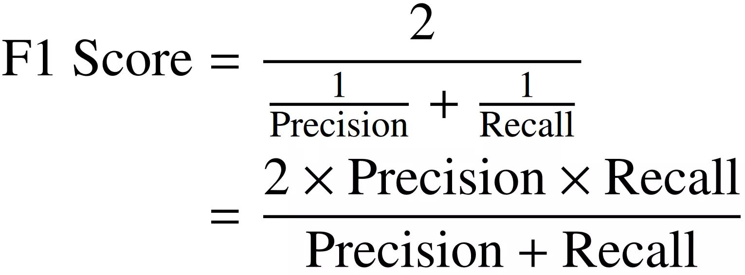
3. F1-Score: The F1-score is a combination of precision and recall, calculated as the harmonic mean of the two. It provides a balance between precision and recall, taking both into account. The F1-score is beneficial for imbalanced datasets as it considers both the positive and negative classes, helping measure the overall performance of the model.
4. Area Under the Curve (AUC-ROC): The receiver operating characteristic (ROC) curve is a graphical representation of the true positive rate (recall) against the false positive rate. The AUC-ROC measures the performance across various classification thresholds, providing an aggregate measure of performance. A higher AUC-ROC indicates a better-performing model in handling the class imbalance.
5. Confusion Matrix: The confusion matrix provides a detailed analysis of the performance of a classification model. It presents a tabular representation of predicted classes against actual classes and shows the true positives, true negatives, false positives, and false negatives. Analyzing the confusion matrix helps understand the model’s performance in correctly classifying instances from both the majority and minority classes.

These evaluation metrics help data scientists assess the performance of models trained on imbalanced data accurately. It is crucial to consider these metrics collectively to gain a comprehensive understanding of the model’s effectiveness in handling the class imbalance and to make informed decisions based on the specific needs of the application.

Accuracy

Accuracy is a commonly used evaluation metric that measures the overall correctness of predictions made by a machine learning model. It is calculated as the ratio of the number of correctly predicted instances to the total number of instances in the dataset. While accuracy is a valuable metric in many classification tasks, it can be misleading when dealing with imbalanced data.

In the context of imbalanced datasets, accuracy alone can give an overly optimistic view of the model’s performance. This is because accuracy does not consider the class imbalance and treats all classes equally. If the majority class dominates the dataset, a model that predicts only the majority class will achieve high accuracy, while performing poorly on the minority class.

Consider a credit card fraud detection scenario where fraudulent transactions account for only a small portion of the dataset. If a model predicts all transactions as non-fraudulent, it may achieve a high accuracy due to the overwhelming majority of non-fraudulent transactions. However, such a model is of little use in predicting the minority class accurately, the fraudulent transactions.

Therefore, while accuracy provides an overall measure of correctness, it should be interpreted cautiously in the context of imbalanced data. It is essential to complement accuracy with other evaluation metrics that focus on the minority class to obtain a more accurate understanding of the model’s performance.

Despite its limitations, accuracy can still be useful as a benchmark or a starting point for model evaluation. It provides a general indication of the model’s performance and can help compare different models. However, it should be used in conjunction with metrics such as precision, recall, F1-score, AUC-ROC, and confusion matrix to gain a more comprehensive evaluation of a model’s performance on imbalanced data.

Precision and Recall

Precision and recall are evaluation metrics commonly used for imbalanced data classification tasks. They provide valuable insights into the model’s performance in correctly predicting the positive instances (minority class) and are particularly useful when the focus is on detecting the minority class accurately.

Precision measures the proportion of correctly predicted positive instances out of all instances predicted as positive. It is calculated as the ratio of true positives to the sum of true positives and false positives. A high precision indicates low false positive rate, implying that the model has correctly identified a high percentage of actual positive instances.

Recall, also known as sensitivity or true positive rate, measures the proportion of correctly predicted positive instances out of all actual positive instances. It is calculated as the ratio of true positives to the sum of true positives and false negatives. A high recall indicates a low false negative rate, meaning that the model has successfully captured a high percentage of the actual positive instances.

The interplay between precision and recall is crucial, especially in imbalanced data scenarios. A model with high precision correctly predicts the positive instances with high confidence, minimizing the inclusion of false positives. On the other hand, a high recall ensures that the model captures a substantial portion of the actual positive instances, minimizing the exclusion of false negatives.

It is important to strike a balance between precision and recall based on the specific requirements of the application. In some cases, precision may be more critical, prioritizing the avoidance of false positives. For example, in a medical diagnosis, it is crucial to minimize the false positive rate to avoid misdiagnosis. In other cases, recall may be more important, especially when the goal is to capture as many positive instances as possible, such as in fraud detection.

Evaluating precision and recall together provides a more comprehensive assessment of the model’s performance, specifically with regards to the minority class. By analyzing the precision-recall trade-off, data scientists can make informed decisions about the model and any necessary adjustments needed to achieve the desired balance between precision and recall.

F1-Score

The F1-score is a widely used evaluation metric that combines both precision and recall into a single value. It provides a balanced assessment of a model’s performance on imbalanced data by considering both the ability to correctly predict positive instances (precision) and the ability to capture all actual positive instances (recall).

The F1-score is calculated as the harmonic mean of precision and recall, balancing their contributions. It ranges from 0 to 1, where a value of 1 indicates perfect precision and recall, and a value of 0 indicates poor performance.

The harmonic mean accounts for the imbalanced nature of the data since it emphasizes the impact of lower values. In other words, if either precision or recall is low, the F1-score will be closer to zero, reflecting the overall performance in handling the minority class.

Consider a scenario where the aim is to build a model for detecting a rare disease. In this case, accurately predicting positive cases (high precision) and capturing as many actual positive cases as possible (high recall) are equally important. The F1-score provides a single metric that balances both aspects, allowing for an evaluation of the model’s effectiveness in handling the imbalanced data.

The F1-score is particularly useful when the class distribution is heavily imbalanced, as it can reveal the true performance of the model on the minority class. It provides a robust evaluation measure that is not easily influenced by the dominating majority class.

However, it is important to note that the F1-score is not always the most appropriate metric for all scenarios. In cases where precision or recall needs to be prioritized over the other, other evaluation metrics like precision or recall should be analyzed independently. The choice of the most appropriate metric should be based on the specific goals and requirements of the application.

Overall, the F1-score is a valuable metric for evaluating the performance of machine learning models in imbalanced data settings. It provides a balanced assessment of precision and recall and helps gauge the model’s effectiveness in making accurate predictions for both the majority and minority classes.

Area Under the Curve (AUC-ROC)

The Area Under the Curve (AUC) of the Receiver Operating Characteristic (ROC) curve is a popular evaluation metric for imbalanced data classification tasks. The ROC curve visualizes the trade-off between the true positive rate (sensitivity) and the false positive rate (1-specificity) for different classification thresholds.

The AUC-ROC metric provides an aggregated measure of the model’s performance across various classification thresholds. It quantifies the ability of the model to distinguish between the positive and negative classes, irrespective of the specific threshold chosen.

The AUC-ROC ranges from 0 to 1, where a value of 1 indicates a perfect classification model, and a value of 0.5 suggests random guessing or a model that performs no better than chance.

A high AUC-ROC value implies that the model has a higher true positive rate and lower false positive rate, indicating good performance in correctly classifying instances from the minority class while keeping the misclassification rate of the majority class low.

The AUC-ROC metric is advantageous for imbalanced data because it is less influenced by the class distribution. It assesses the model’s overall discriminatory power, evaluating its ability to correctly rank positive and negative instances even in scenarios where the majority class dominates the dataset.

Moreover, the AUC-ROC allows for easy comparison between different models. When comparing two or more models, the model with a higher AUC-ROC generally indicates better performance in handling the class imbalance.

However, it is essential to note that the AUC-ROC metric does not provide insights into the costs associated with misclassifications or the optimal classification threshold. Depending on the specific application, a different threshold might be more appropriate, even though it affects the AUC-ROC value. Therefore, it is crucial to consider other evaluation metrics, such as precision, recall, or F1-score, alongside the AUC-ROC when making decisions about model performance.

Overall, the AUC-ROC is a valuable evaluation metric for imbalanced data. It provides an aggregated assessment of the model’s discriminatory power, allowing for performance comparison and offering insights into the model’s ability to handle the class imbalance effectively.

Confusion Matrix

The confusion matrix is a tabular representation that provides detailed insights into the performance of a machine learning model on imbalanced data. It allows for a comprehensive analysis of the model’s predictions by comparing the predicted class labels against the actual class labels.

A confusion matrix consists of four key components:

1. True Positives (TP): The number of instances from the positive class (minority class) that are correctly predicted as positive by the model.
2. True Negatives (TN): The number of instances from the negative class (majority class) that are correctly predicted as negative by the model.
3. False Positives (FP): The number of instances from the negative class that are incorrectly predicted as positive by the model.
4. False Negatives (FN): The number of instances from the positive class that are incorrectly predicted as negative by the model.

The confusion matrix provides a breakdown of the model’s performance, allowing for a more nuanced analysis of the errors made by the model. Depending on the specific goals and requirements of the application, different aspects of the confusion matrix can be of interest.

For example, in a medical diagnostic scenario, false negatives (instances incorrectly predicted as negative when they are positive) can be more critical than false positives (instances incorrectly predicted as positive when they are negative). Misclassifying a disease as non-disease can have severe consequences, while misclassifying a non-disease as disease may lead to further testing, but not necessarily harm the patient.

The confusion matrix further facilitates the calculation of other evaluation metrics such as accuracy, precision, and recall. These metrics can be derived directly from the values in the confusion matrix, providing a more in-depth understanding of the model’s performance on both the majority and minority classes.

By analyzing the confusion matrix, data scientists can gain insights into the specific types of errors made by the model and identify potential areas for improvement. It helps identifying whether the model is biased towards the majority class or properly captures the minority class instances.

In summary, the confusion matrix is a powerful tool for evaluating the performance of machine learning models on imbalanced data. It provides a detailed breakdown of predictions and their correctness, enabling a more granular analysis of the model’s performance on the minority and majority classes.

Conclusion

Dealing with imbalanced data is a significant challenge in machine learning. The prevalence of the majority class and the underrepresentation of the minority class can lead to biased models and inaccurate predictions. However, by utilizing appropriate techniques and evaluation metrics, data scientists can effectively handle imbalanced data and improve the performance of their machine learning models.

In this article, we explored several techniques for handling imbalanced data. Resampling techniques such as oversampling and undersampling can adjust the class distribution to achieve a more balanced dataset. Algorithmic techniques, such as adjusting class weights and modifying algorithms, offer ways to account for the class imbalance during model training. Cost-sensitive learning assigns different misclassification costs to different classes, addressing the inherent disparities in the data. Ensemble methods, including bagging, boosting, and stacking, leverage multiple models to improve performance and robustness.

Furthermore, we discussed evaluation metrics specifically designed for imbalanced data. Accuracy, while commonly used, does not adequately reflect the performance on minority classes. Precision and recall provide insights into the ability to correctly identify positive instances and capture all actual positives. The F1-score combines precision and recall into a single metric. The AUC-ROC measures the overall discriminatory power of the model. Lastly, the confusion matrix offers a detailed analysis of predictions, showcasing the types of errors made by the model.

It is important to note that no single technique or evaluation metric is universally superior. The choice of techniques and metrics depends on the specific dataset, problem, and requirements of the application. Careful experimentation and validation are necessary to identify the most appropriate approach for each imbalanced data scenario.

By addressing the challenges associated with imbalanced data and employing suitable techniques and evaluation metrics, data scientists can enhance the performance and reliability of their machine learning models. This allows for more accurate predictions, improved decision-making, and better outcomes in domains where imbalanced data is prevalent.