Introduction
Machine learning has revolutionized the way we approach data analysis and make predictions. One crucial aspect of the machine learning process is feature engineering. In simple terms, feature engineering involves selecting, transforming, and creating new variables (features) from the available data to improve the performance of a machine learning model.
Feature engineering is a critical step that directly impacts the accuracy and efficiency of a machine learning algorithm. It aims at maximizing the predictive power of the selected features and reducing noise or irrelevant information in the dataset.
Effective feature engineering can significantly enhance the performance of machine learning models, while poor feature engineering can lead to suboptimal or even misleading results. It requires a combination of domain knowledge, creativity, and data exploration skills to identify and engineer the most relevant features for a particular problem.
In this article, we will explore the importance of feature engineering and delve into various techniques used to improve the quality and effectiveness of feature engineering in machine learning.
First, we will discuss the importance of feature engineering in machine learning. Then, we will explore different types of feature engineering techniques, including data cleaning and preprocessing, handling missing data, dealing with categorical variables, numerical transformations, feature scaling, feature extraction, dimensionality reduction, feature selection, and feature creation.
This article aims to provide a comprehensive overview of the different techniques involved in feature engineering and the role they play in enhancing the performance of machine learning models. By the end of this article, you will have a solid understanding of feature engineering and be equipped with practical knowledge to apply these techniques in your own machine learning projects.
Definition of Feature Engineering
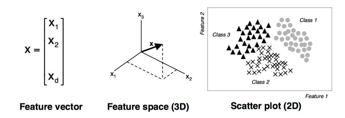
Feature engineering is the process of selecting, transforming, and creating new variables (features) from the available data to improve the performance of machine learning models. It involves extracting meaningful insights from raw data by creating features that capture the underlying patterns and relationships.
At its core, feature engineering is about transforming and representing data in a way that allows machine learning algorithms to effectively learn from it. It goes beyond simply collecting the data and involves careful consideration of which features are most relevant and informative for the task at hand.
The goal of feature engineering is to enhance the predictive power of machine learning models by providing them with input features that are more representative of the underlying patterns in the data. This is achieved by manipulating the existing features or creating new features based on the available data.
Feature engineering encompasses a wide range of techniques and strategies, including data cleaning and preprocessing, handling missing data, dealing with categorical variables, numerical transformations, feature scaling, feature extraction, dimensionality reduction, feature selection, and feature creation.
By carefully engineering the features, we can improve the accuracy, efficiency, and interpretability of machine learning models. It enables us to extract meaningful information, reduce noise or irrelevant data, and capture the important characteristics of the dataset.
Feature engineering is a crucial step in the machine learning pipeline as it directly impacts the performance of the models. Properly engineered features can significantly improve the model’s ability to generalize and make accurate predictions on unseen data.
However, feature engineering is also an iterative process that requires experimentation, domain knowledge, and a deep understanding of the data. It involves continuous refinement and examination of feature combinations to ensure optimal performance.
In summary, feature engineering plays a vital role in machine learning by transforming raw data into informative features that enhance the predictive power of models. It involves a variety of techniques aimed at improving the quality and effectiveness of features, ultimately leading to more accurate and reliable machine learning models.
Importance of Feature Engineering
Feature engineering is a critical step in the machine learning process, and its importance cannot be overstated. While machine learning algorithms can analyze data and make predictions, the quality of the features used as input greatly influences the accuracy and performance of the models. Here are some key reasons why feature engineering is essential:
1. Improved Model Performance: Feature engineering allows us to transform raw data into meaningful features that better represent the underlying patterns in the data. By selecting or creating relevant features, we can provide the model with more informative inputs, leading to improved predictive accuracy and overall model performance.
2. Noise Reduction: Not all features in a dataset are relevant for making accurate predictions. In fact, some variables may introduce noise or irrelevant information that can adversely affect model performance. Feature engineering helps identify and remove or transform noisy features, allowing the model to focus only on the most significant and informative variables.
3. Capturing Non-linear Relationships: In many real-world scenarios, the relationships between the input variables and the target variable may not be linear. Feature engineering enables us to create new features that capture non-linear relationships, such as polynomial features, interaction terms, or other non-linear transformations. This expands the model’s ability to capture complex patterns and enhances its predictive capabilities.
4. Handling Missing Data: Real-world datasets often contain missing values, which can cause problems for machine learning algorithms. Feature engineering techniques like imputation can help handle missing data by filling in the gaps with appropriate values. This ensures that valuable information is not lost and allows the model to make use of the complete dataset.
5. Dealing with Categorical Variables: Many datasets contain categorical variables, which require special handling for machine learning models. Feature engineering techniques such as one-hot encoding, target encoding, or ordinal encoding help transform categorical variables into a format that the model can easily understand and utilize for predictions.
6. Dimensionality Reduction: Some datasets may have a large number of features, which can lead to computational challenges and overfitting. Feature engineering techniques like principal component analysis (PCA) or other dimensionality reduction methods can help reduce the number of features while retaining most of the relevant information, making the model more efficient and reducing the risk of overfitting.
7. Interpretability: Feature engineering also plays a crucial role in improving the interpretability of machine learning models. By creating features that are easy to understand and relate to the problem domain, we can gain insights into how the model is making predictions and explain its decisions to stakeholders and domain experts.
In summary, feature engineering is a fundamental step in the machine learning process, enabling us to transform raw data into meaningful and informative features. By carefully selecting, transforming, and creating features, we can improve model performance, reduce noise, capture non-linear relationships, handle missing data, deal with categorical variables, reduce dimensionality, and enhance interpretability. These benefits collectively contribute to building more accurate, efficient, and reliable machine learning models.
Types of Feature Engineering Techniques
Feature engineering encompasses a range of techniques to manipulate, transform, and create new variables from the available data. These techniques help maximize the predictive power of machine learning models and extract meaningful insights. Here are some key types of feature engineering techniques:
1. Data Cleaning and Preprocessing: This involves techniques such as removing duplicates, handling outliers, and normalizing or standardizing data. Data cleaning ensures that the dataset is free from inconsistencies and prepares it for further feature engineering steps.
2. Handling Missing Data: Missing data can pose challenges for machine learning models. Feature engineering techniques like imputation, where missing values are filled in using statistical measures, allow the dataset to be used effectively without losing valuable information.
3. Handling Categorical Variables: Categorical variables need to be transformed into numerical representations for most machine learning models. One-hot encoding creates a binary column for each category, while target encoding or ordinal encoding assigns numeric values based on target variables or the order of categories.
4. Numerical Transformations: Numeric features can be transformed to better conform to the assumptions of the models. Techniques such as logarithmic transformations, square root transformations, or box-cox transformations can be applied to create linear relationships or reduce the impact of outliers.
5. Feature Scaling: Scaling features to a similar range can improve the stability and convergence speed of models. Techniques like standardization (mean = 0, standard deviation = 1) or normalization (scaling to a specific range) can be used to achieve this scaling.
6. Feature Extraction: Feature extraction involves deriving new features from existing ones using techniques such as mathematical functions, statistical measures, or domain-specific knowledge. For example, extracting the day of the week from a date-time feature or calculating the length of text can provide valuable information.
7. Dimensionality Reduction: High-dimensional datasets can lead to computational challenges and overfitting. Techniques like principal component analysis (PCA) or linear discriminant analysis (LDA) can reduce the number of features while preserving most of the important information, improving model efficiency.
8. Feature Selection: Selecting the most relevant features helps reduce model complexity and improve interpretability. Techniques like univariate selection, recursive feature elimination, or feature importance from tree-based models can be used to identify and select the most informative features.
9. Feature Creation: Creating new features by combining existing ones can capture important interactions and non-linear relationships. Techniques like polynomial features, interaction terms, or binning can be applied to introduce valuable features into the dataset.
By employing these various feature engineering techniques, data scientists and machine learning practitioners can enhance the quality and effectiveness of the features used by machine learning models. Each technique serves a specific purpose in addressing different challenges and extracting the most relevant information from the dataset.
Data Cleaning and Preprocessing
Data cleaning and preprocessing is an essential step in feature engineering as it ensures that the dataset is free from inconsistencies and prepares it for further analysis. This process involves handling duplicates, outliers, and ensuring the data is in a suitable format for machine learning models. Here are some key techniques used in data cleaning and preprocessing:
1. Handling Duplicates: Duplicates in the dataset can skew the results and introduce bias. It’s important to detect and remove duplicate records to ensure the data is accurate and representative of the underlying population. This can be done by identifying duplicate rows based on all or a subset of features.
2. Handling Outliers: Outliers are extreme data points that deviate significantly from the majority of the observations. These can occur due to measurement errors or genuine anomalous events. Depending on the context, outliers can be removed, transformed, or assigned a specific value to minimize their impact on the analysis.
3. Data Formatting: Ensuring that the data is in the correct format is crucial for effective analysis. This may involve converting data types (e.g., transforming strings to numeric values), standardizing date formats, or normalizing the representation of categorical variables (e.g., capitalizing or converting to lowercase).
4. Handling Missing Data: Missing data is a common challenge in real-world datasets. Missing values can be handled by various techniques, including imputation. Imputation involves filling in the missing values with estimates based on statistical measures like mean, median, or mode, or using more advanced techniques like regression or k-nearest neighbors.
5. Removing Irrelevant or Redundant Features: Not all features in the dataset may be useful for the modeling process. Irrelevant or redundant features can increase model complexity and lead to overfitting. It is important to carefully evaluate and remove such features to improve model performance.
6. Dealing with Skewed Data: Skewed data, where the distribution of values is not symmetrical, can affect the performance of machine learning models. Techniques like log transformation or power transformations (e.g., Box-Cox) can be applied to mitigate the impact of skewness and make the data more suitable for modeling.
7. Handling Inconsistent Data: Inconsistent data can arise due to data entry errors, data integration from different sources, or inconsistencies in coding conventions. It is important to identify and address such inconsistencies, either by correcting the data or by adopting consistent conventions for representation.
8. Normalizing or Scaling: Normalizing or scaling the data ensures that features are on a similar scale, preventing certain features from dominating others during the modeling process. Common techniques include standardization (e.g., mean = 0, standard deviation = 1) or normalization (scaling to a specific range).
Data cleaning and preprocessing lay the foundation for effective feature engineering. By addressing issues such as duplicates, outliers, missing data, inconsistent formatting, and irrelevant features, the dataset becomes more reliable, accurate, and suitable for further analysis. These steps contribute to the overall quality and effectiveness of the features used in machine learning models.
Handling Missing Data
Missing data is a common challenge in real-world datasets and can affect the performance and accuracy of machine learning models. It is important to appropriately handle missing data to ensure that valuable information is not lost and that the model can effectively learn from the available data. Here are some common techniques for handling missing data:
1. Deleting Rows or Columns: In cases where the amount of missing data is relatively small compared to the overall dataset, deleting rows or columns with missing values can be a viable option. This approach is suitable when the missing data is believed to be random and removing them will not introduce bias into the analysis.
2. Imputation: Imputation involves filling in the missing values with estimated values. The choice of imputation method depends on the nature of the data and the missing data mechanism. Common imputation techniques include mean imputation (replacing missing values with the mean value of the feature), median imputation (replacing missing values with the median value of the feature), mode imputation (replacing missing values with the most frequent value of the feature), or regression imputation (predicting the missing values based on the relationship with other features).
3. Creating a Missing Indicator: Instead of imputing missing values, another approach is to create an additional binary variable that indicates whether a value is missing or not. This approach can help the model capture any potential patterns or relationships associated with missing data.
4. Time-Series Interpolation: For datasets with a time component, missing values can be interpolated based on the values before and after the missing point in time. This approach is useful when missing data is believed to follow a temporal pattern.
5. Multiple Imputation: Multiple imputation involves creating multiple imputed datasets by generating plausible values for the missing data multiple times. Each imputed dataset is then used to perform separate analyses, and the results are combined to obtain overall estimates. Multiple imputation takes into account the uncertainty associated with imputing missing values and provides more reliable estimates compared to single imputation methods.
6. Domain-Specific Imputation: Depending on the context of the data, domain knowledge can guide the imputation of missing values. For example, if the missing data is related to a specific category or group, imputing with the most common value for that group may be a reasonable approach.
7. Avoiding Uninformative Features: In some cases, if a feature has a high proportion of missing values, it may be better to exclude that feature from the analysis altogether. The presence of too many missing values can make the feature unreliable and introduce noise into the model.
Handling missing data is crucial to ensure the integrity and reliability of the dataset used for machine learning. The choice of technique depends on factors such as the amount of missing data, the missing data mechanism, the nature of the data, and the specific problem at hand. By appropriately addressing missing data, we can avoid bias, preserve valuable information, and improve the accuracy and performance of machine learning models.
Handling Categorical Variables
Categorical variables play an important role in many datasets, but they require special handling in machine learning models. Since most machine learning algorithms are designed to work with numerical data, categorical variables need to be transformed into a format that can be easily understood and processed. Here are some common techniques for handling categorical variables:
1. One-Hot Encoding: One-hot encoding is a popular technique used to convert categorical variables into a binary format. It creates new binary columns, each representing a unique category in the original variable. The new columns have values of 1 or 0, indicating the presence or absence of a specific category, respectively. One-hot encoding enables machine learning algorithms to interpret categorical variables as numerical inputs, without assigning any ordinal relationship between categories.
2. Target Encoding: Target encoding, also known as mean encoding or likelihood encoding, replaces each category value with the average value of the target variable for that category. This technique captures the relationship between the categorical variable and the target variable. However, target encoding may lead to overfitting if not properly regularized.
3. Ordinal Encoding: Ordinal encoding assigns integer values to categories based on their order or rank. This is suitable when there is an inherent order or hierarchy among the categories. For example, assigning values of 1, 2, 3 to the categories “low,” “medium,” and “high” would capture the relationship of increasing values.
4. Binary Encoding: Binary encoding represents each category as a binary code, using a combination of 0s and 1s. Binary encoding reduces the dimensionality of the encoded variables relative to one-hot encoding, making it more memory-efficient and sometimes more computationally efficient.
5. Count Encoding: Count encoding replaces each category with the count of occurrences of that category in the dataset. This technique is helpful when the frequency or abundance of a category provides meaningful information.
6. Feature Hashing: Feature hashing, or the “hashing trick,” is a technique that converts categorical variables into a fixed number of features using a hash function. This technique can efficiently handle high-dimensional categorical variables and is particularly useful when the number of categories is large.
7. Label Encoding: Label encoding assigns a unique numeric value to each category, typically starting from 0 or 1. Label encoding is suitable for categorical variables with no inherent order or when encoding is not expected to introduce any meaningful relationships between categories. However, it is important to ensure that the assigned numeric values do not imply any ordinal relationship.
By appropriately handling categorical variables, we enable machine learning models to effectively utilize these features and capture the valuable information they provide. The choice of technique depends on the specific characteristics of the categorical variable, the nature of the data, and the requirements of the machine learning algorithm.
Numerical Transformations
Numerical transformations are a key feature engineering technique used to manipulate and modify numerical variables to better conform to the assumptions of machine learning models. These transformations help improve the relationships between variables, handle skewness, and reduce the influence of outliers. Here are some common numerical transformations:
1. Logarithmic Transformation: Applying a logarithmic transformation, such as taking the natural logarithm or base 10 logarithm, can help make the data less skewed and more normally distributed. This transformation is particularly useful when the data spans a wide range, and a few extreme values are influencing the distribution.
2. Square Root Transformation: Taking the square root of a variable can help stabilize the variance, especially when the data is positively skewed or exhibits heteroscedasticity. This transformation can also be useful when the relationship between the variable and the target is expected to be more linear.
3. Box-Cox Transformation: The Box-Cox transformation is a family of power transformations that automatically selects the optimal transformation parameter lambda (λ) to normalize the data as much as possible. This transformation can handle different shapes of data distributions and is widely used to improve feature normality.
4. Min-Max Scaling: Min-Max scaling, also known as normalization, rescales the data to a specific range, usually between 0 and 1. This transformation ensures that all features have a similar scale and prevents certain features from dominating others due to their original magnitude.
5. Standardization: Standardization, also known as Z-score normalization, transforms the data to have a mean of zero and a standard deviation of one. This transformation makes the data more suitable for models that assume a Gaussian distribution and allows for easier interpretability of the model’s coefficients.
6. Binning: Binning involves dividing a continuous variable into discrete bins or intervals. This transformation can help capture non-linear relationships or patterns that exist between the variable and the target. Binning can be done using equal width intervals, equal frequency intervals, or based on domain knowledge.
7. Winsorization: Winsorization involves replacing extreme values, such as outliers, with less extreme values to reduce their influence on the analysis. This transformation can be helpful when outliers are suspected to be due to data measurement errors or data entry mistakes.
8. Rank Transformation: Rank transformation replaces the original values with their ranks. This is useful when the exact values are not as important as the relative ordering or when dealing with non-parametric statistical tests.
Each of these numerical transformations serves a specific purpose in feature engineering, allowing for better representation of the data and improved performance of machine learning models. The choice of transformation depends on the data distribution, the relationship with the target variable, and the assumptions of the modeling technique being used.
Feature Scaling
Feature scaling is a crucial step in feature engineering that ensures all features in a dataset are on a similar scale. It is essential because many machine learning algorithms are sensitive to the magnitude of the features, and having features on different scales can affect model performance and convergence. Here are some common techniques used for feature scaling:
1. Min-Max Scaling (Normalization): Min-Max scaling, also known as normalization, rescales the data to a specific range, typically between 0 and 1. This transformation subtracts the minimum value of the feature and divides by the range (maximum value minus minimum value). Min-Max scaling ensures that all features have the same magnitude and can be particularly useful when the absolute values of the features are important.
2. Standardization (Z-score normalization): Standardization transforms the data to have a mean of zero and a standard deviation of one. It subtracts the mean of the feature from each value and divides by the standard deviation. Standardization preserves the shape of the distribution and is suitable when the underlying data follows a Gaussian distribution. It also enables easy comparison between different features as they are all on the same scale.
3. Robust Scaling: Robust scaling is a method that uses a robust measure of scale to rescale the data. Instead of using the mean and standard deviation, it uses the median and interquartile range (IQR). Robust scaling is suitable when the dataset contains outliers or is not normally distributed. By using the median and IQR, it reduces the influence of outliers on the scaling process.
4. Logarithmic Transformation: In some cases, applying a logarithmic transformation to the data can improve scaling. This transformation can help when the data has a skewed distribution with a long tail. Taking the logarithm of the values compresses the scale and makes the data more symmetrical.
Choosing the appropriate scaling technique depends on the characteristics of the dataset and the requirements of the machine learning algorithm. It is important to note that feature scaling should generally be applied to the independent features and not the target variable.
Feature scaling brings several benefits to the modeling process. It prevents certain features from dominating others due to their original scale, improves the stability and convergence speed of models, and can make the interpretation of model coefficients more meaningful. By scaling the features, machine learning algorithms can treat all variables equally and make more informed predictions.
Feature Extraction
Feature extraction is a technique in feature engineering that involves deriving new features from existing ones. It aims to capture the most informative aspects of the data and reduce the dimensionality of the feature space. Feature extraction can be particularly useful when dealing with high-dimensional or complex datasets. Here are some common techniques used for feature extraction:
1. Principal Component Analysis (PCA): PCA is a popular technique used for dimensionality reduction. It converts a set of possibly correlated variables into a set of linearly uncorrelated variables called principal components. These components are ordered in terms of their variance, with the first component capturing the most variance in the data. By selecting a subset of the principal components, the dimensionality of the data can be significantly reduced while preserving most of the essential information.
2. Independent Component Analysis (ICA): ICA is a statistical technique that separates a multivariate signal into additive subcomponents. It assumes that the observed variables are linear mixtures of the unknown source components. ICA can be used for feature extraction when the goal is to identify underlying independent sources contributing to the observations, such as in audio signal processing or blind source separation tasks.
3. Linear Discriminant Analysis (LDA): LDA is a dimensionality reduction technique that maximizes the separability between classes in a supervised learning setting. It seeks to find a projection that maximizes the ratio of between-class scatter to within-class scatter. LDA is commonly used in classification problems to reduce the dimensionality while maximizing the class separability.
4. Non-negative Matrix Factorization (NMF): NMF is a dimensionality reduction technique that decomposes a non-negative matrix into the product of two non-negative matrices. It is particularly useful for documents or image data as it can discover latent topics or patterns. NMF extracts meaningful components that are non-negative and interpretable.
5. Wavelet Transform: The wavelet transform is a mathematical technique used for time-frequency analysis. It decomposes a signal into a series of wavelet coefficients at different scales and positions. Wavelet analysis can reveal both localized and global characteristics of the data, making it useful for feature extraction in signal processing or image analysis tasks.
6. Fourier Transform: The Fourier transform is a mathematical technique that decomposes a signal into a combination of sine and cosine wave components. It represents the signal in the frequency domain, revealing periodic patterns and frequencies. Fourier analysis is widely used in signal processing and feature extraction tasks where frequency content is important.
7. Feature Selection: Feature selection is another form of feature extraction that aims to select a subset of the most relevant features based on their importance or contribution to the target variable. This can be done through statistical measures like univariate feature selection, recursive feature elimination, or through the use of feature importance from tree-based models.
Feature extraction techniques enable us to reduce the dimensionality of the dataset, eliminate redundant or irrelevant features, and capture the most informative aspects of the data. By extracting meaningful features, machine learning models can focus on the most relevant information and make more accurate predictions.
Dimensionality Reduction
Dimensionality reduction is a critical technique in feature engineering that aims to reduce the number of features in a dataset while preserving the most important information. It is especially useful for high-dimensional datasets where the number of features is large compared to the number of observations. Here are some common techniques used for dimensionality reduction:
1. Principal Component Analysis (PCA): PCA is a widely used technique for dimensionality reduction. It identifies the directions (principal components) that capture the maximum variance in the data. By selecting a subset of the principal components that explain a significant amount of the total variance, PCA reduces the dimensionality while retaining the essential information. PCA is particularly effective when there is high correlation among the original features.
2. Linear Discriminant Analysis (LDA): LDA is a dimensionality reduction technique that aims to maximize the separability between classes in a supervised learning setting. It identifies the linear combination of features that best separates the classes while reducing the dimensionality. LDA is commonly used in classification problems where the goal is to find a lower-dimensional representation that maximizes the class separability.
3. Non-negative Matrix Factorization (NMF): NMF is a dimensionality reduction technique that decomposes a non-negative matrix into the product of two non-negative matrices. It aims to represent the data as a combination of non-negative components, which can be interpreted as latent features. NMF is especially useful for capturing the underlying structure in non-negative data, such as text or image data, and reducing dimensionality while preserving interpretability.
4. t-SNE: t-SNE (t-Distributed Stochastic Neighbor Embedding) is a technique that reduces the dimensionality of the data while preserving the local structure and similarity relationships. It is particularly effective for visualizing high-dimensional data in a lower-dimensional space. t-SNE is often used for exploratory data analysis or to gain insights into the underlying structure of the data.
5. Autoencoders: Autoencoders are neural network models designed for unsupervised learning. They can be used for dimensionality reduction by learning a compressed representation of the input data. The input and output of the autoencoder are the same, and the middle layer (encoding layer) serves as a low-dimensional representation of the data. Autoencoders are capable of capturing non-linear relationships and can be used for both linear and non-linear dimensionality reduction.
6. Feature Selection: Feature selection is a technique used to select a subset of the most relevant features from the original dataset. It eliminates redundant or irrelevant features, effectively reducing dimensionality. Feature selection can be performed based on various criteria, such as statistical measures, correlation analysis, or the use of feature importance from tree-based models.
Dimensionality reduction techniques are valuable in feature engineering as they help to overcome the curse of dimensionality and improve model efficiency by reducing computational complexity. By removing irrelevant or redundant features, these techniques enable machine learning models to focus on the most informative aspects of the data, leading to better generalization and improved predictive performance.
Feature Selection
Feature selection is a technique used in feature engineering to select a subset of the most relevant features from the original dataset. It aims to eliminate redundant or irrelevant features and improve model performance, interpretability, and efficiency. Feature selection can be performed based on various criteria and algorithms. Here are some common techniques used for feature selection:
1. Univariate Selection: Univariate selection involves selecting features based on their individual performance in relation to the target variable. Statistical measures like chi-square test, ANOVA F-test, or mutual information can be used to score each feature, and the top-k features with the highest scores are selected. This technique is straightforward and computationally efficient but does not capture feature interactions.
2. Recursive Feature Elimination (RFE): RFE is an iterative feature selection algorithm that starts with all features and eliminates the least important ones based on their importance scores. It relies on the training performance of a machine learning model and progressively removes features until a specified number or criteria are met. RFE is especially useful for models that provide feature importance scores, such as tree-based models.
3. Embedded Methods: Embedded methods incorporate feature selection as part of the model training process. Different algorithms, such as Lasso (L1 regularization), Ridge (L2 regularization), or Elastic Net, penalize certain features and encourage sparsity. These methods simultaneously optimize model performance and select the most important features, which reduces overfitting and enhances interpretability.
4. Feature Importance: Feature importance is determined by tree-based models, such as decision trees or random forests. These models assign importance scores to each feature based on how much they contribute to reducing impurity or improving predictive performance. Features with high importance scores are selected, and the rest can be discarded. Feature importance provides insights into the relative significance of each feature and helps identify the most informative ones.
5. Correlation Analysis: Correlation analysis measures the strength and direction of the linear relationship between features and the target variable or between features themselves. High correlations among features indicate redundancy. By selecting one representative feature from strongly correlated pairs, we can reduce the dimensionality and eliminate multicollinearity, which can affect model stability and interpretation.
6. Domain Knowledge: Domain knowledge is often valuable in feature selection. Understanding the problem and the dataset allows for the identification of relevant features based on prior knowledge or expert insights. By selecting features that are likely to have a strong relationship with the target variable, we can improve the model’s performance and interpretability.
Feature selection reduces the dimensionality of the dataset, improves model efficiency, mitigates overfitting, and enhances interpretability. It helps to focus on the most informative features, reducing noise and improving generalization. The choice of feature selection technique depends on the dataset, the model, and the specific requirements of the problem at hand. By selecting the most relevant features, we can build more accurate and efficient machine learning models.
Feature Creation
Feature creation is a powerful technique in feature engineering that involves creating new features from the existing ones to capture more relevant information and improve model performance. It allows us to extract insights, capture non-linear relationships, and enhance the discriminative power of the data. Here are some common techniques used for feature creation:
1. Polynomial Features: Polynomial features involve creating new features through polynomial combinations of the original features. For example, if we have a feature x, creating polynomial features of degree 2 would include x^2 and x^3. This technique helps capture non-linear relationships between variables, allowing models to capture more complex patterns and interactions.
2. Interaction Terms: Interaction terms are created by multiplying two or more features together. This technique takes into account the combined effect of the features on the target variable. For example, in a dataset with features x1 and x2, we can create an interaction term as x1 * x2 to capture their combined impact on the target variable.
3. Binning: Binning involves grouping numerical values into intervals or bins. This technique is useful when the precise values of the features are less important than the ranges they belong to. Binning can help capture non-linear relationships and handle outliers. It also allows for the interpretation of continuous variables as categorical variables.
4. Encoding Cyclical Features: Cyclical features, such as time or compass directions, exhibit periodic patterns. Instead of treating them as continuous variables, we can encode them as cyclical features. For example, encoding months as sine and cosine transformations can retain the cyclical nature of the features and preserve the order and relationship between different months.
5. Text Feature Engineering: Text data requires a different approach for feature creation. Techniques such as bag-of-words, TF-IDF (Term Frequency-Inverse Document Frequency), n-grams, and word embeddings can be used to transform text into numerical features that machine learning models can understand. These techniques capture the presence of specific words or phrases and the semantic relationships between them.
6. Derived Features: Derived features can be created by applying mathematical operations or functions to the original features. For example, calculating the logarithm or square root of a feature can transform the data and uncover non-linear relationships. These derived features provide additional insights and may improve model performance.
7. Domain-Specific Features: Domain-specific knowledge is invaluable in feature creation. Expert understanding of the problem and the dataset can guide the creation of features that are most relevant to the specific domain. By incorporating domain knowledge, we can create features that capture specific aspects of the problem and enhance the model’s performance.
The process of feature creation should be guided by an understanding of the problem, the dataset, and the specific requirements of the model. It is an iterative process that requires experimentation and domain expertise. By creating new features, we can extract more meaningful information from the data and build more accurate and robust machine learning models.
Target Encoding
Target encoding is a technique used in feature engineering to convert categorical variables into meaningful numerical representations by encoding them with the target variable. It is particularly useful when dealing with categorical variables in predictive modeling tasks. Target encoding helps capture the relationship between the category levels and the target variable, providing valuable information to machine learning models. Here’s how target encoding is typically performed:
1. Split the dataset into different folds or chunks to avoid data leakage.
2. For each category in the categorical feature:
a. Calculate the average target value (e.g., mean or median) for that category in the training set.
b. Encode each category level with the computed average target value.
3. Replace the original categorical feature with the encoded numerical feature in the training set.
4. To avoid overfitting, use the target encoding applied to the training set for encoding the categorical feature in the test set.
Target encoding provides several benefits in predictive modeling:
1. Incorporating Categorical Variables: Machine learning models typically work well with numerical data. Target encoding allows us to utilize categorical variables in a meaningful way, contributing valuable information to the models.
2. Capturing Relationship: By encoding categories with the target variable, target encoding captures the relationship between the categorical feature and the target. This can be particularly useful when categorical variables have a strong influence on the target and can significantly enhance model performance.
3. Handling High Cardinality: High cardinality refers to categorical variables with a large number of unique categories. Target encoding can effectively handle high cardinality features by summarizing the information of each category in relation to the target variable.
4. Preserving Information: Target encoding retains the information from the categorical feature in a numerical form. This ensures that the encoded feature retains the original characteristics and patterns, contributing to the model’s ability to learn and make accurate predictions.
5. Addressing Outliers: Target encoding can help mitigate the impact of outliers on model performance. By using aggregate statistics (e.g., mean or median) instead of individual observations, target encoding provides a more robust representation of the categorical variable.
Caution should be exercised while using target encoding to avoid potential pitfalls:
1. Data Leakage: It is crucial to perform target encoding in a manner that avoids data leakage. Leakage occurs when information from the validation or test set is used during encoding. To prevent leakage, target encoding should be applied separately to the training and test sets without consulting any future information.
2. Overfitting: Target encoding can lead to overfitting, especially when there is a high degree of imbalance in the target variable or when encoding rare categories. Appropriate regularization techniques, such as adding noise or smoothing parameters, can be applied to alleviate the risk of overfitting.
Target encoding is a powerful technique in feature engineering, allowing us to leverage the information carried by categorical variables. While it requires careful implementation to avoid leakage and overfitting, target encoding can significantly enhance the performance and interpretability of machine learning models.
One-Hot Encoding
One-hot encoding is a popular technique used in feature engineering to represent categorical variables as binary vectors. It allows machine learning models to effectively interpret and utilize categorical data. One-hot encoding creates new binary variables for each category in the original feature, indicating the presence or absence of that category in the observation. Here’s how one-hot encoding is typically performed:
1. Identify categorical variables in the dataset that need to be one-hot encoded.
2. For each categorical feature:
a. Create binary variables called dummy variables, equal to the number of distinct categories in the feature.
b. Assign a value of 1 to the appropriate dummy variable if the observation belongs to that category.
c. Assign a value of 0 to all other dummy variables.
3. Replace the original categorical feature with the set of binary dummy variables in the dataset.
One-hot encoding offers several advantages in feature engineering:
1. Preserving Categorical Information: One-hot encoding retains the information from the categorical feature in a numerical format. It ensures that each category is represented by a distinct binary variable, allowing the model to understand and utilize the categorical information effectively.
2. Handling Categorical Variables: Many machine learning algorithms require numerical inputs. One-hot encoding enables us to use categorical variables as input features in these algorithms, where numerical representations are more appropriate.
3. Overcoming Non-Ordinal Categories: One-hot encoding is particularly useful when dealing with non-ordinal categories. By creating separate binary variables for each category, we avoid imposing an arbitrary order on the categories.
4. Avoiding Implying False Relationships: By representing categorical variables with binary variables, one-hot encoding ensures that no false ordinal relationships are introduced. Each category is mutually exclusive, and there is no inherent order conveyed by the encoding.
One consideration for one-hot encoding is the potential increase in the dimensionality of the dataset, especially when dealing with high-cardinality categorical variables. This can lead to a large number of columns in the dataset, which may impact model training time and performance. Dimensionality reduction techniques, such as feature selection or principal component analysis, can be applied to mitigate this issue.
It is important to note that one-hot encoding should be applied carefully to avoid the “dummy variable trap.” This occurs when one or more dummy variables can be perfectly predicted from the remaining dummy variables. To avoid multicollinearity, one of the dummy variables should be dropped or left out as the reference category.
One-hot encoding is a widely used technique in feature engineering for representing categorical variables as binary vectors. It enables effective utilization of categorical information in machine learning models, promoting accurate predictions and insights from the data.
Polynomial Features
Polynomial features are created through a process called polynomial expansion in feature engineering. This technique involves generating new features by raising existing features to different powers and multiplying them. It allows machine learning models to capture non-linear relationships between variables, enhancing their capability to model complex patterns and interactions. Here’s how polynomial features are typically generated:
1. Identify the numerical features in the dataset that will be used for polynomial expansion.
2. For each selected feature, generate new features by combining it with other features and raising them to different powers, such as 2, 3, or higher.
3. Combine the original features with the newly generated polynomial features to create an expanded feature set.
By incorporating polynomial features, several benefits can be achieved:
1. Capturing Non-Linear Relationships: Polynomial features enable machine learning models to capture non-linear relationships between variables. By introducing higher-order terms and their interactions, polynomial features can better represent complex patterns and interactions in the data, allowing models to make more accurate predictions.
2. Improving Model Flexibility: Polynomial expansion increases the flexibility of models, particularly those that assume a linear relationship between variables. By introducing polynomial features, models can capture non-linearities and improve their ability to fit the training data more accurately.
3. Accounting for Interaction Effects: Interaction effects occur when the combination of two or more features has a different impact on the target variable compared to their individual contributions. By including interaction terms in the polynomial features, models can capture these interactions and better understand their influence.
4. Avoiding Underfitting: Underfitting occurs when a model is too simple to capture the underlying relationships in the data. By incorporating polynomial features, models become more expressive and capable of capturing complex relationships. This reduces the risk of underfitting and allows models to better represent the data.
It is important to consider the potential impact of polynomial features on model complexity and interpretability. Generating higher-degree polynomial features can significantly increase the number of features and may lead to increased computational requirements and potential overfitting. Regularization techniques, such as L1 or L2 regularization, can be employed to mitigate overfitting when using polynomial features.
Polynomial features enable machine learning models to capture non-linear relationships and interactions in the data, enhancing their performance and predictive capabilities. By introducing higher-order terms, models can better represent the complexity of real-world phenomena and improve their generalization to unseen data.
Binning
Binning, also known as discretization, is a technique in feature engineering that involves grouping numerical values into intervals or bins. It converts continuous variables into categorical or ordinal features, allowing machine learning models to capture non-linear relationships or handle outliers. Binning is especially useful when the precise values of the features are less important than the range or category to which they belong. Here’s how binning is typically performed:
1. Determine the appropriate number and size of bins for the feature. This can be based on domain knowledge, statistical methods, or data exploration.
2. Divide the range of the feature into equally sized intervals (equal width binning) or intervals with an equal number of observations (equal frequency binning).
3. Assign each value to the respective bin based on its value falling within the interval boundaries.
4. Replace the original numerical feature with the assigned categorical or ordinal bins.
Binning provides several advantages in feature engineering:
1. Capturing Non-Linear Relationships: Binning allows machine learning models to capture non-linear relationships between variables. By converting continuous features into discrete intervals, models can better represent complex patterns or non-linear trends that may not be obvious from the raw numerical data.
2. Handling Outliers: Binning can help address the impact of outliers by grouping extreme values into specific bins. This allows models to focus on the data distribution within each bin and reduces the influence of outliers that might otherwise skew the results or affect model performance.
3. Simplifying Complexity: Binning simplifies the representation of continuous variables by converting them into a small number of discrete categories or ordinal values. This reduction in complexity can improve model interpretability, especially when specific ranges or categories have a significant impact on the target variable.
4. Facilitating Interpretation: Binning enables easy interpretation of continuous features as categorical or ordinal variables. It allows non-technical stakeholders to understand the relationship between the features and the target variable in a more straightforward manner.
It’s important to note that the choice of binning method and the number of bins should be carefully considered. If the number of bins is too small, important information may be lost, while too many bins may lead to overfitting. Statistical techniques and domain knowledge can help determine the appropriate binning strategy for the specific problem and dataset.
Binning is a versatile technique in feature engineering that allows machine learning models to effectively handle continuous variables. By converting numerical features into categorical or ordinal bins, models gain the ability to capture non-linear relationships, handle outliers, simplify complexity, and enhance interpretability.
Interaction Terms
Interaction terms, also known as interaction effects, are a powerful technique in feature engineering that allows machine learning models to capture the combined influence and relationships between two or more features. It involves creating new features through the multiplication or combination of existing features. Interaction terms enable models to capture non-additive effects and understand how the joint presence of certain features affects the target variable. Here’s how interaction terms are typically created:
1. Identify the predictor variables that may have a joint influence or interaction effect on the target variable.
2. Create new features by multiplying or combining these predictor variables. For example, if we have features x1 and x2, we can create an interaction term as x1 * x2.
3. Incorporate the interaction terms into the feature set used for training the machine learning model.
By incorporating interaction terms, we can achieve several benefits:
1. Capturing Non-Additive Relationships: Interaction terms enable models to capture non-additive relationships between variables. Interactions can reveal complex dependencies that exist when two or more features coexist, allowing models to account for the joint impact of multiple features on the target variable.
2. Incorporating Contextual Information: Interaction terms help models understand how the relationship between predictor variables changes based on different contexts or conditions. They provide contextual information about how the impact of one feature varies with the presence or absence of another, leading to more accurate predictions.
3. Uncovering Synergistic Effects: Interaction terms can reveal synergistic effects where the joint influence of two or more features is greater than the sum of their individual contributions. These synergistic effects may not be evident when considering the features individually but become apparent when their interactions are taken into account.
4. Enhancing Model Flexibility: Interaction terms increase the flexibility and expressiveness of machine learning models by incorporating additional feature combinations. This allows models to capture complex relationships and improve their ability to fit the training data closely, leading to better predictions on unseen data.
It is important to consider potential challenges when working with interaction terms:
1. Curse of Dimensionality: When adding interaction terms, the dimensionality of the feature space increases exponentially. This can lead to an increased risk of overfitting when working with limited amounts of data. Proper regularization techniques, feature selection, or dimensionality reduction methods should be employed to mitigate this challenge.
2. Interpretability: Interaction terms can complicate model interpretation since the relationships between features may become more intricate. It is important to strike a balance between model complexity and interpretability, ensuring that the interaction terms are meaningful and aligned with the problem domain.
Interaction terms are a valuable technique in feature engineering, enabling machine learning models to capture non-linear relationships and understand the joint influence of features. By incorporating interaction terms, models gain the ability to capture complex patterns and improve their predictive performance.
Conclusion
Feature engineering is a crucial aspect of machine learning that involves transforming and creating features from the available data. It plays a vital role in enhancing the performance, accuracy, and interpretability of machine learning models. Throughout this article, we have explored a range of feature engineering techniques and their importance in the modeling process.
We started by understanding the definition of feature engineering, which involves selecting, transforming, and creating new variables to improve model performance. We discussed the significance of feature engineering in machine learning, emphasizing its ability to maximize the predictive power of models and reduce noise or irrelevant information in the dataset.
We then delved into various types of feature engineering techniques, including data cleaning and preprocessing, handling missing data, dealing with categorical variables, numerical transformations, feature scaling, feature extraction, dimensionality reduction, feature selection, feature creation, target encoding, one-hot encoding, polynomial features, binning, and interaction terms. Each of these techniques serves a specific purpose in manipulating and optimizing features to make them more informative and suitable for machine learning models.
Finally, we highlighted the importance of careful implementation and consideration of factors such as data leakage, overfitting, model complexity, and interpretability when applying feature engineering techniques. It is essential to strike a balance between extracting meaningful information and preventing potential pitfalls that can arise from flawed feature engineering practices.
In conclusion, feature engineering is a fundamental step in the machine learning process. It empowers data scientists to transform raw data into informative features, capture complex relationships, and improve model performance. By applying the appropriate techniques and leveraging domain knowledge, feature engineering enables us to better understand the data, make accurate predictions, and extract insights to drive informed decision-making.