Introduction
When it comes to machine learning, achieving optimal performance is the goal. This is where optimization techniques play a crucial role. In the realm of machine learning algorithms, optimization refers to the process of finding the best set of parameters that minimize or maximize a specific objective function. By fine-tuning these parameters, models can be trained to make accurate predictions and deliver optimal results.
Optimization in machine learning is not only about improving performance but also about finding the right balance between accuracy and efficiency. It involves striking a trade-off between fitting the training data perfectly and generalizing well to unseen data. Different optimization algorithms are employed to find the optimal values of parameters, ensuring that the model achieves its intended purpose.
In this article, we will dive into the world of optimization in machine learning, exploring key concepts and popular algorithms. Understanding these optimization techniques is crucial for any data scientist or machine learning practitioner looking to improve their models’ performance.
Before we delve deeper, it’s important to note that optimization in machine learning is a vast field with numerous approaches, algorithms, and concepts. This article aims to provide an overview and introduction to optimization techniques frequently used in machine learning tasks.
Now, let’s embark on our journey to uncover the secrets of optimization in machine learning!
Understanding Optimization in Machine Learning
Optimization in machine learning involves the process of iteratively adjusting the parameters of a model to minimize the error or loss function. The goal is to find the best set of parameter values that lead to the most accurate predictions on unseen data. To understand optimization in machine learning, it’s essential to grasp some key concepts.
One fundamental concept in optimization is the objective function. The objective function, also known as the loss function or cost function, measures the discrepancy between the predicted output of a model and the actual output. The optimization algorithm aims to minimize this function to achieve the best possible model performance.
Another crucial concept is the search space. The search space refers to the range of possible values that the parameters can take. The task of optimization is to explore this search space and find the combination of parameter values that result in the lowest possible value of the objective function.
Optimization in machine learning relies on the use of gradients to determine the direction and magnitude of parameter updates. Gradients provide information about the rate of change of the objective function with respect to each parameter. By following the gradient, optimization algorithms can iteratively update the parameter values in a way that leads to the desired global minimum of the objective function.
Understanding optimization also involves recognizing the trade-off between underfitting and overfitting. Underfitting occurs when the model is too simple and fails to capture the underlying patterns in the data. Overfitting, on the other hand, happens when the model becomes too complex and performs well on the training data but poorly on unseen data. Optimization aims to strike a balance between these two extremes by finding the optimal set of parameters that achieve good generalization performance.
Lastly, it’s important to note that optimization is an iterative process. The algorithms repeat the steps of evaluating the objective function, computing gradients, and updating the parameters until a stopping criterion is met. This could be a maximum number of iterations, reaching a certain level of improvement in the objective function, or other predefined conditions.
Now that we have a basic understanding of what optimization entails in machine learning, let’s explore some of the key algorithms used in this process.
Key Concepts in Optimization
To effectively navigate the world of optimization in machine learning, it’s essential to familiarize ourselves with some key concepts. These concepts lay the foundation for understanding and implementing optimization algorithms. Let’s explore them in more detail.
Objective Function: The objective function, also known as the loss function or cost function, quantifies the discrepancy between the predicted output of a model and the actual output. It provides a measure of how well the model is performing. The goal of optimization is to minimize this function, finding the parameter values that yield the lowest possible value.
Search Space: The search space refers to the range of possible values that the parameters of a model can take. Optimizing the model involves exploring this space to find the combination of parameter values that result in the best performance. The size and complexity of the search space depend on the number and nature of the parameters.
Gradients: Gradients are vital in optimization as they provide information about the rate of change of the objective function with respect to each parameter. By computing and analyzing gradients, optimization algorithms can determine the direction and magnitude of parameter updates. Gradients show the way toward the desired global minimum of the objective function.
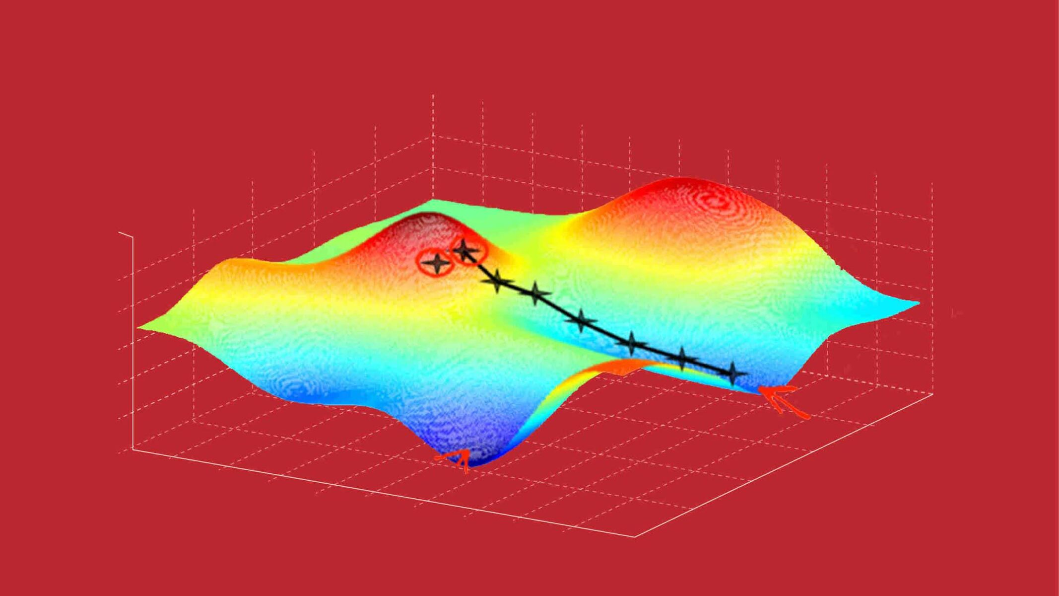
Local Minima and Global Minima: The objective function can have multiple local minima, which are points where the function reaches a low value in the vicinity. The goal of optimization is to find the global minimum, which is the lowest point in the entire search space. Addressing the challenge of avoiding local minima is crucial for effective optimization.
Convergence: Convergence refers to the point at which the optimization algorithm stops and declares that the optimal solution has been found. It can be determined by reaching a maximum number of iterations, achieving a predefined level of improvement in the objective function, or other stopping criteria. Convergence ensures that the algorithm does not run indefinitely.
Regularization: Regularization is a technique used to prevent overfitting in machine learning models. It is especially important in optimization as it helps control the complexity of the model by adding a penalty term to the objective function. Regularization encourages the model to generalize well to unseen data, striking a balance between fitting the training data and avoiding overfitting.
By grasping these key concepts in optimization, we can better appreciate the inner workings of various optimization algorithms. In the following sections, we will explore some of the popular optimization algorithms used in machine learning tasks.
Gradient Descent
Gradient descent is one of the most popular and widely used optimization algorithms in the field of machine learning. It is an iterative optimization algorithm that aims to find the minimum of an objective function by repeatedly adjusting the model’s parameters in the direction opposite to the gradient.
The basic idea behind gradient descent is to start with an initial set of parameter values and iteratively update these values in small steps, guided by the negative gradient of the objective function. By following the gradient, the algorithm moves in the direction of steepest descent, progressively reducing the value of the objective function.
There are different variations of gradient descent, depending on the amount of data used in each iteration. Some common types include:
- Batch Gradient Descent: In batch gradient descent, the algorithm computes the gradient of the objective function using the entire training dataset. It then updates the parameters based on this gradient and repeats the process until convergence is reached. Batch gradient descent can be computationally expensive for large datasets, as it requires evaluating the objective function for all training examples in each iteration.
- Stochastic Gradient Descent: Stochastic gradient descent (SGD) is a variation of gradient descent that randomly selects a single training example at each iteration. The algorithm computes the gradient of the objective function for that example and updates the parameters accordingly. SGD is computationally more efficient than batch gradient descent, especially for large datasets. However, due to the randomness introduced by the single example, it can exhibit more noise during the optimization process.
- Mini-Batch Gradient Descent: Mini-batch gradient descent is a compromise between batch gradient descent and stochastic gradient descent. It randomly samples a small subset, or mini-batch, of the training data at each iteration. The algorithm computes the gradient using this mini-batch and updates the parameters. Mini-batch gradient descent strikes a balance between computational efficiency and stability during the optimization process.
Gradient descent has its strengths and limitations. It is a versatile algorithm that can be applied to a wide range of optimization problems. However, it can sometimes get trapped in local minima and may take longer to converge. Additionally, gradient descent is sensitive to the learning rate, which determines the size of the steps taken during parameter updates. Choosing an appropriate learning rate is crucial to ensure effective optimization.
Despite these considerations, gradient descent remains a fundamental optimization algorithm in machine learning. Its simplicity, flexibility, and effectiveness make it a go-to choice for many optimization tasks. As we delve into other optimization algorithms, we will see how they build upon the principles of gradient descent to address its limitations and enhance the optimization process.
Stochastic Gradient Descent
Stochastic gradient descent (SGD) is a variant of the gradient descent algorithm that offers computational efficiency in large-scale machine learning tasks. Unlike batch gradient descent, which uses the entire training dataset to compute the gradient, SGD updates the model parameters using a single randomly selected training example at each iteration.
The key advantage of SGD is its ability to handle large datasets without requiring excessive computational resources. By using only one example per iteration, SGD reduces the computational burden associated with evaluating the objective function for the entire dataset. This makes it particularly useful when dealing with massive datasets that would be impractical to process using batch gradient descent.
While SGD offers computational efficiency, it introduces some challenges as well. One of the main challenges is the high level of algorithmic noise. Since SGD updates the parameters based on a single training example, the gradient estimate obtained from that one example may not be a perfect representation of the overall gradient. This randomness can lead to oscillations and hinder the convergence of the algorithm.
To mitigate the noise and stabilize the optimization process, learning rate scheduling techniques are often employed. These techniques adjust the learning rate over time, allowing larger steps at the beginning of training when the parameters are far from the optimal solution and gradually decreasing the step size as the optimization progresses. Common learning rate scheduling techniques include step decay, exponential decay, and adaptive learning rate methods such as AdaGrad and RMSprop.
Another consideration in SGD is the order in which the training examples are presented. By randomly shuffling the training data before each epoch, SGD prevents the algorithm from getting stuck in a specific order of examples and gives it a chance to explore different parts of the search space. Furthermore, shuffling helps to prevent bias in training and ensures that the model learns from a diverse range of examples.
SGD is a popular choice in deep learning, where models often have millions or even billions of parameters and training data can be extremely large. By leveraging the benefits of SGD, deep learning models can be trained efficiently, enabling the exploration of complex patterns and structures in the data.
Despite its limitations, such as the noise introduced by a single training example and the need for careful tuning of learning rates, stochastic gradient descent remains a powerful and widely adopted optimization algorithm in machine learning. Its ability to handle large-scale datasets efficiently makes it an essential tool in many real-world applications.
Batch Gradient Descent
Batch gradient descent is a classic optimization algorithm used in machine learning. It updates the model parameters by computing the gradient of the objective function using the entire training dataset in each iteration. This approach contrasts with stochastic gradient descent, which operates on a single randomly selected training example, and mini-batch gradient descent, which uses a subset of the training data.
Batch gradient descent offers some advantages over the stochastic counterparts. First, it provides a more accurate estimate of the true gradient since it considers the complete dataset. This can lead to smoother convergence and more stable optimization overall. Additionally, batch gradient descent can take larger steps during parameter updates, which may result in faster convergence in certain situations.
However, batch gradient descent also comes with its drawbacks. The main challenge lies in computational efficiency. Computing the gradient using the entire dataset can be time-consuming and memory-intensive, especially for large-scale machine learning tasks.
Despite its computational drawbacks, batch gradient descent is still widely used in practice, particularly when the dataset fits in memory or when computational resources are sufficient to handle the workload. It is especially popular in scenarios where accurate gradient estimates are crucial for achieving optimal performance, such as in small-sized datasets or situations where the risk of getting stuck in local minima is high.
Batch gradient descent allows for fine-grained control over the learning process. The choice of learning rate plays a vital role in determining the step sizes during parameter updates. If the learning rate is set too high, the algorithm can overshoot the optimal solution, potentially diverging. On the other hand, a learning rate that is too small can result in slow convergence or getting stuck in local minima.
To address the computational challenges and reduce memory usage, various techniques have been developed, such as mini-batch gradient descent and its variants. These methods strike a balance between the efficiency of stochastic gradient descent and the accuracy of batch gradient descent by computing the gradient on a subset of the training data at each iteration.
In summary, batch gradient descent is a fundamental optimization algorithm that provides accurate gradient estimates by utilizing the entire training dataset. Although it may not be the most efficient option for large-scale machine learning tasks, it remains a valuable tool in scenarios where accurate optimization and convergence to the global minimum are crucial.
Mini-Batch Gradient Descent
Mini-batch gradient descent is a popular variant of the gradient descent algorithm that combines the advantages of both batch gradient descent and stochastic gradient descent. In mini-batch gradient descent, the model parameters are updated based on the gradient computed on a small randomly selected subset, or mini-batch, of the training data at each iteration.
Mini-batch gradient descent strikes a balance between the efficiency of stochastic gradient descent and the accuracy of batch gradient descent. By computing the gradient on a mini-batch of examples, mini-batch gradient descent reduces the computational burden compared to batch gradient descent while still providing a more accurate estimate of the true gradient than stochastic gradient descent.
The size of the mini-batch is a hyperparameter that needs to be carefully chosen. A smaller mini-batch size introduces more noise in the gradient estimate due to the limited number of examples used. On the other hand, a larger mini-batch size can lead to slower convergence or even getting stuck in sharp minima as the algorithm is less likely to escape such areas.
The mini-batch gradient descent algorithm also offers several practical advantages. First, it can leverage the parallel processing capabilities of modern hardware, such as GPUs, by processing multiple examples simultaneously. This makes mini-batch gradient descent a suitable choice for training large-scale models efficiently.
Another benefit of mini-batch gradient descent is that it exhibits smoother convergence compared to stochastic gradient descent. By considering a mini-batch of examples in each iteration, the algorithm reduces the variance in the gradient estimate, leading to a more stable optimization process.
Selecting an appropriate learning rate is crucial in mini-batch gradient descent. A learning rate that is too high can cause the algorithm to overshoot the optimal solution, while a learning rate that is too low can result in slow convergence. Adaptive learning rate techniques such as AdaGrad, RMSprop, or Adam can be employed to automatically adjust the learning rate during training and improve convergence efficiency.
Mini-batch gradient descent is widely used in practice, especially in deep learning, where large-scale models and datasets are common. It offers a good balance between computational efficiency and stable convergence, making it an effective optimization algorithm for various machine learning tasks.
In summary, mini-batch gradient descent provides a compromise between the efficiency of stochastic gradient descent and the accuracy of batch gradient descent. By updating the model parameters based on a mini-batch of examples, mini-batch gradient descent combines computational efficiency with more accurate gradient estimates, making it a popular choice in many machine learning applications.
Common Optimization Algorithms
Optimization in machine learning encompasses a wide range of algorithms, each designed to address specific challenges and optimize different types of models. Let’s explore some of the most common optimization algorithms used in the field:
Gradient Descent: Gradient descent is a fundamental optimization algorithm that iteratively adjusts the model parameters by following the negative gradient of the objective function. It comes in various forms, including batch gradient descent, stochastic gradient descent, and mini-batch gradient descent. Gradient descent is widely used due to its simplicity and effectiveness in finding the global minimum of the objective function.
Adam: Adam (Adaptive Moment Estimation) is an adaptive optimization algorithm that combines ideas from both momentum and RMSprop. It maintains an adaptive learning rate for each parameter and adjusts the learning rate based on the magnitude of gradients. Adam is known for its fast convergence and robustness across various types of neural network architectures.
Adagrad: Adagrad (Adaptive Gradient) is an optimization algorithm that adapts the learning rate to the individual parameters. It gives larger updates to infrequent parameters and smaller updates to frequent parameters, effectively addressing the problem of scaling the learning rate. Adagrad is particularly useful in sparse feature learning scenarios and has been successful in natural language processing and recommendation systems.
RMSprop: RMSprop (Root Mean Square Propagation) is an adaptive learning rate algorithm that divides the learning rate for each parameter by the root mean square (RMS) of the historical gradient magnitudes. It dampens the oscillations and improves convergence in the presence of noisy gradients. RMSprop is commonly used in deep learning tasks.
AdaDelta: AdaDelta is an adaptive learning rate algorithm that aims to overcome the need for manual tuning of learning rates. It utilizes a running average of squared gradients to adaptively adjust the learning rate. AdaDelta has been shown to converge faster than other methods in certain scenarios and is particularly effective when training deep networks.
Adamax: Adamax is a variant of Adam that replaces the second moment estimator with the infinite norm (max norm). It has been shown to be less sensitive to the choice of hyperparameters and performs well in training models with sparse gradients, such as those encountered in text data or generative models.
LBFGS: LBFGS (Limited-memory Broyden-Fletcher-Goldfarb-Shanno) is a popular optimization algorithm for problems with a large number of parameters. It approximates the inverse Hessian matrix of the objective function using limited memory, making it memory-efficient for high-dimensional problems. LBFGS is commonly used in scenarios where the objective function is smooth and the computational resources are limited.
These are just a few examples of the many optimization algorithms available in the machine learning literature. The choice of the algorithm depends on several factors, including the nature of the problem, the size of the dataset, the computational resources available, and the specific requirements of the model being optimized.
By understanding and utilizing these common optimization algorithms, machine learning practitioners can efficiently train models and achieve improved performance across a variety of tasks and domains.
Choosing the Right Optimization Algorithm
With several optimization algorithms available, choosing the right one for a specific machine learning task can significantly impact the performance and convergence of the model. Consider the following factors when selecting an optimization algorithm:
Problem Type: The nature of the problem at hand can influence the choice of optimization algorithm. For example, if the objective function is convex, algorithms like gradient descent or its variations may be suitable. Non-convex problems, on the other hand, may require more sophisticated algorithms that can handle multiple local optima, such as Adam or LBFGS.
Data Size: The size of the dataset can affect the efficiency of optimization algorithms. While batch gradient descent may work well for smaller datasets that fit into memory, stochastic gradient descent or mini-batch gradient descent are often preferred for larger datasets due to their computational efficiency.
Computational Resources: The availability of computational resources should also be taken into account. Algorithms like Adam or RMSprop may require more memory and computational power than simpler methods like stochastic gradient descent. Consider the capabilities of the hardware and the scalability requirements of the problem when selecting an optimization algorithm.
Model Complexity: The complexity of the model being optimized can influence the choice of algorithm. Deep learning models with numerous parameters and layers often benefit from adaptive optimization algorithms like Adam or Adagrad, as they can handle the complexity and optimize the model parameters efficiently.
Convergence Speed: The speed at which an algorithm converges to an optimal solution is another important factor. Some algorithms, like stochastic gradient descent and its variations, may converge faster due to their ability to adaptively update the parameters based on individual training examples. However, faster convergence may come at the expense of increased noise or oscillations in the optimization process.
Hyperparameter Sensitivity: Different optimization algorithms have their own sets of hyperparameters that need to be tuned for optimal performance. Some algorithms, such as Adam or Adagrad, have default hyperparameters that work well in many scenarios. However, fine-tuning the hyperparameters based on the specific problem and dataset can further improve the optimization process.
Choosing the right optimization algorithm requires careful consideration of these factors. It often involves experimentation and comparison of different algorithms on the specific problem to identify the one that leads to the best convergence, performance, and stability.
It’s worth mentioning that some machine learning frameworks and libraries provide default optimization algorithms that work well out of the box for many scenarios. However, understanding the underlying principles and characteristics of different optimization algorithms can help practitioners make informed decisions and customize the optimization process based on the specific requirements of their models and datasets.
Conclusion
Optimization plays a vital role in machine learning, enabling models to achieve their maximum potential. By fine-tuning the parameters of a model, optimization algorithms seek to minimize the objective function and improve performance.
In this article, we explored the key concepts of optimization, including the objective function, search space, gradients, and the trade-off between underfitting and overfitting. We delved into various optimization algorithms, such as gradient descent, stochastic gradient descent, batch gradient descent, and mini-batch gradient descent.
Different optimization algorithms have their strengths and weaknesses. Batch gradient descent provides accurate gradient estimates but can be computationally intensive for larger datasets. Stochastic gradient descent is computationally efficient, but the use of individual examples introduces more noise. Mini-batch gradient descent strikes a balance between the two by using a subset of training examples.
We also discussed other popular optimization algorithms, including Adam, Adagrad, RMSprop, AdaDelta, Adamax, and LBFGS. Each algorithm offers unique features and advantages suited for different scenarios, such as adaptive learning rates, handling sparsity, or memory efficiency.
When choosing the right optimization algorithm, considerations such as problem type, data size, computational resources, model complexity, convergence speed, and hyperparameter sensitivity are all crucial. It often requires experimentation and tuning to find the algorithm that best suits the specific requirements of the problem.
It’s important to note that optimization in machine learning is a dynamic field with ongoing research and development. New algorithms and techniques constantly emerge, offering improved performance and efficiency. Staying up to date with the latest advancements can help practitioners continually enhance their models’ optimization process.
In conclusion, optimization is a crucial aspect of machine learning, allowing models to achieve optimal performance. By understanding the various optimization algorithms and selecting the right one for a given task, practitioners can optimize their models effectively and unlock their true potential.