How To Train A Machine Learning Model In Python

Introduction

Welcome to the fascinating world of machine learning! In this digital age, where data is abundant and algorithms can analyze and learn from it, machine learning has become an essential tool for many industries. Whether it’s predicting customer behavior, automated recommendation systems, or detecting fraud, machine learning models have the power to extract meaningful insights and make accurate predictions.

In this article, we will explore the fundamentals of training a machine learning model using Python, one of the most popular programming languages for data analysis and machine learning. We will dive into the process of setting up the environment, loading and preparing the dataset, choosing an appropriate algorithm, training the model, and evaluating its performance.

Before we get started, it’s important to have a basic understanding of what machine learning is. At its core, machine learning is a subset of artificial intelligence that focuses on the development of algorithms that allow computers to learn and make decisions without explicit programming. Instead, they learn from patterns and data.

Machine learning models rely on historical data to identify patterns and relationships, which they use to generate predictions or make informed decisions. These models are trained using a variety of techniques, such as supervised learning, unsupervised learning, and reinforcement learning.

Python is an excellent language choice for machine learning due to its simplicity, extensive libraries, and strong community support. Some of the most popular libraries for machine learning in Python include scikit-learn, TensorFlow, and Keras. These libraries provide a wide range of algorithms and tools to facilitate the training and evaluation of machine learning models.

Throughout this article, we will use a dataset as an example to walk you through the process of training a machine learning model. By the end, you should feel confident in your ability to apply these techniques to your own datasets and solve real-world problems using machine learning algorithms.

So, without further ado, let’s dive into the exciting world of machine learning and discover how to train a model that can learn from data and make intelligent predictions.

Understanding Machine Learning

Before we delve into the process of training a machine learning model, it’s essential to have a clear understanding of what machine learning is and how it works. At a high level, machine learning is a branch of artificial intelligence that focuses on the development of algorithms that enable computers to learn from and make predictions or decisions based on data.

Machine learning models are designed to automatically identify patterns, relationships, and trends in data without being explicitly programmed. This is accomplished by using statistical techniques and algorithms that iteratively learn from training data to improve their performance over time.

There are three main types of machine learning: supervised learning, unsupervised learning, and reinforcement learning.

• Supervised Learning: In supervised learning, the training dataset is labeled, meaning that the input data is paired with corresponding correct output labels. The model learns from the labeled examples to make predictions on unseen data. Classification and regression problems are common applications of supervised learning.
• Unsupervised Learning: Unsupervised learning involves training a model on unlabeled data. The goal is to find hidden patterns, clusters, or structures in the data. Clustering and dimensionality reduction are examples of unsupervised learning techniques.
• Reinforcement Learning: Reinforcement learning is a different approach in which an agent interacts with an environment and learns to make decisions through trial and error. The agent receives rewards or punishments based on its actions, allowing it to learn an optimal sequence of actions to maximize rewards.

To train a machine learning model, we typically follow a standard workflow:

1. Acquire and preprocess the dataset.
2. Split the dataset into a training set and a test set.
3. Select an appropriate algorithm or model architecture.
4. Train the model using the training set.
5. Evaluate the model’s performance using the test set.
6. Tune the model’s hyperparameters to optimize its performance.
7. Once satisfied with the model’s performance, deploy it to make predictions on new, unseen data.

By understanding the fundamentals of machine learning and the different types of learning approaches, we can lay a solid foundation for training accurate and reliable models. Now that you have a grasp of the basics, let’s move on to setting up the environment to start training our own machine learning model.

Setting up the Environment

Before we can start training a machine learning model, we need to set up our development environment. Python, with its vast libraries and tools for data analysis and machine learning, is an excellent choice for this task. Let’s go through the steps to ensure we have everything we need to proceed.

1. Install Python: If you don’t already have Python installed, head over to the official Python website and download the latest version compatible with your operating system. Follow the installation instructions, and make sure to add Python to your system’s PATH variable.

2. Install a Package Manager: While Python comes with its package manager, pip, it is recommended to install a higher-level package manager such as Anaconda or Miniconda. These package managers make it easier to manage and install the various libraries and dependencies required for machine learning projects.

3. Create a Virtual Environment: Creating a virtual environment is good practice to keep your project’s dependencies isolated from other Python installations. Use the following command to create a virtual environment:

conda create –name myenv
conda activate myenv

4. Install Required Libraries: The next step is to install the libraries we will be using for machine learning. The most popular libraries are NumPy, Pandas, and scikit-learn. Run the following commands to install these libraries:

pip install numpy pandas scikit-learn

5. Install Jupyter Notebooks (Optional): Jupyter Notebooks are a fantastic tool for data exploration, visualization, and prototyping machine learning models. To install Jupyter Notebooks, run:

pip install jupyter

6. Test the Installation: Once the libraries are installed, it’s a good idea to test the installation by launching a Jupyter Notebook or an integrated development environment (IDE) such as PyCharm or Spyder. Open a new notebook and try importing the libraries we just installed (e.g., numpy, pandas). If there are no import errors, it means the installation was successful.

Congratulations! You have now set up your machine learning environment. With Python and the required libraries installed, you are ready to start training your own machine learning models. In the next section, we will dive into the process of loading and preparing the dataset for training.

Importing the Required Libraries

Now that we have our environment set up, it’s time to import the necessary libraries that we will be using throughout our machine learning project. These libraries provide various tools and functions to simplify data handling, feature engineering, model training, and evaluation. Let’s explore the key libraries we need to import.

NumPy: NumPy is a fundamental library for scientific computing in Python. It provides support for large, multi-dimensional arrays and matrices, along with a collection of mathematical functions to perform computations efficiently. We will use NumPy extensively for data manipulation and numerical operations.

Pandas: Pandas is a versatile library for data manipulation and analysis. It offers powerful data structures, such as DataFrames, that allow us to work with structured data efficiently. With Pandas, we can load datasets, perform data cleaning and preprocessing tasks, and carry out exploratory data analysis effectively.

Scikit-learn: Scikit-learn is a popular machine learning library that provides a wide range of algorithms and tools for classification, regression, clustering, and more. It offers a consistent interface and allows us to easily implement machine learning models for our projects. Scikit-learn also provides tools for data preprocessing, feature selection, and model evaluation.

Matplotlib and Seaborn: Matplotlib and Seaborn are visualization libraries that enable us to create informative and visually appealing plots and charts. Matplotlib is a comprehensive library that provides low-level plotting functions, while Seaborn is built on top of Matplotlib and offers a higher-level interface with stylish and visually pleasing default settings.

Let’s import these libraries:

python
import numpy as np
import pandas as pd
import sklearn
import matplotlib.pyplot as plt
import seaborn as sns

By importing these libraries, we now have access to powerful tools and functions that will facilitate our machine learning journey. With NumPy and Pandas, we can load and manipulate data efficiently, while Scikit-learn provides a wide range of algorithms and evaluation metrics. Matplotlib and Seaborn will help us visualize and explore the data in a meaningful way.

In the next section, we will dive into loading and preparing the dataset, which is a crucial step before training our machine learning model.

Loading and Preparing the Dataset

Once we have imported the necessary libraries, the next step is to load and prepare the dataset. The dataset serves as the foundation for training our machine learning model. It contains the input features (independent variables) and the corresponding target variable (dependent variable) that we want to predict.

The specific steps for loading and preparing the dataset may vary depending on the format and structure of the data. However, the general process involves the following:

1. Loading the Dataset: We need to obtain the dataset in a format that can be easily read and analyzed by our machine learning algorithms. Common file formats include CSV (Comma Separated Values), JSON (JavaScript Object Notation), and Excel. We can use the Pandas library to read in the data using appropriate functions like read_csv() or read_json().
2. Exploratory Data Analysis (EDA): Exploratory Data Analysis is a critical step in understanding the dataset. We can use various Pandas functions to get an overview of the data, such as head(), describe(), and info(). Visualizations with Matplotlib or Seaborn can also help us identify patterns, distributions, and outliers in the data.
3. Handling Missing Data: In real-world datasets, missing values are common. It’s essential to address missing data before training the model. We can use Pandas functions like isnull(), dropna(), or fillna() to handle missing values appropriately.
4. Handling Categorical Data: Machine learning algorithms typically work with numerical data, so we need to encode categorical data into numerical format. Common techniques include one-hot encoding, label encoding, or ordinal encoding. We can use Scikit-learn’s preprocessing module or Pandas functions like get_dummies() for this task.
5. Feature Scaling: Feature scaling is the process of normalizing or standardizing the numerical features to a consistent range. Scaling ensures that features with different scales do not bias the model. Scikit-learn provides various scaling methods such as StandardScaler, MinMaxScaler, or RobustScaler to transform the data.

By loading and preparing the dataset, we ensure that the data is in a suitable format for training our machine learning model. It allows us to handle missing data, encode categorical variables, and scale the features appropriately. These steps lay the foundation for accurate and reliable model training.

In the next section, we will dive deeper into exploratory data analysis to gain further insights into our dataset.

Exploratory Data Analysis

Exploratory Data Analysis (EDA) is a crucial step in the machine learning pipeline that helps us gain insights into the dataset. It involves analyzing and visualizing the data to understand its characteristics, identify patterns, detect outliers, and determine how the variables relate to each other. By performing EDA, we can make informed decisions in the subsequent steps of our machine learning project.

Let’s explore some common techniques and tools used in EDA:

• Summary Statistics: Computing summary statistics is an effective way to get an overview of the dataset. We can use Pandas functions like describe() to obtain statistical measures such as mean, standard deviation, minimum, maximum, and quartiles for numerical variables. For categorical variables, we can count the unique values using the value_counts() function.
• Data Visualization: Visualizations provide a powerful way to understand the data and identify patterns. Matplotlib and Seaborn libraries offer a wide range of plots, including histograms, box plots, scatter plots, and bar charts. These plots can reveal distributions, relationships, and any potential outliers or anomalies in the data.
• Correlation Analysis: Correlation analysis helps us understand the relationships between variables. We can use Pandas’ corr() function or Seaborn’s heatmap to visualize the correlation matrix. Positive or negative correlation values indicate the strength and direction of the relationship. This analysis can guide feature selection and provide insights into potential multicollinearity issues.
• Feature Engineering: EDA might reveal opportunities for feature engineering. By understanding the data, we can identify new features or transformations that might improve our model’s performance. For example, we might extract date or time-related features from a datetime column, create interaction terms, or derive new variables based on domain knowledge.

Through EDA, we can uncover valuable insights about the dataset and make informed decisions about preprocessing steps. It can help us identify potential issues or biases in the data, assess data quality, and guide us in choosing the most suitable machine learning algorithms for our task.

In the next sections, we will discuss handling missing data and categorical variables, as these are crucial steps in preparing the dataset for training our model.

Handling Missing Data

Handling missing data is an essential step in the data preprocessing phase of a machine learning project. Missing values can cause issues during model training and evaluation, leading to biased or inaccurate results. It is crucial to address missing data to ensure the integrity and reliability of our analysis.

Let’s explore some common strategies for handling missing data:

• Dropping Missing Values: If the number of missing values is relatively small compared to the total dataset, one option is to drop the rows or columns containing missing values. This approach is suitable when missing values are randomly distributed and don’t affect the overall integrity of the dataset. However, caution should be exercised as this can lead to a loss of valuable information.
• Imputation: Imputation is the process of filling in missing values with estimated or predicted values. The choice of imputation method depends on the characteristics of the dataset. Some common imputation techniques include filling missing values with mean, median, or mode values of the respective variable, or using more advanced techniques like regression imputation or K-nearest neighbor imputation.
• Flagging Missing Values: Another approach is to flag missing values as a separate category or code. This can be useful when missing values carry their own significance and may contain valuable information. For categorical variables, missing values can be encoded as “Unknown” or “-1”. For numerical variables, a specific code like -999 can be used.
• Multiple Imputation: Multiple imputation is a technique that generates multiple imputed datasets to handle missing values. Instead of replacing missing values with a single estimate, multiple imputations create several plausible values based on the observed data. This approach accounts for the uncertainty introduced by missing values and provides more accurate estimates for subsequent analyses.

When deciding on the appropriate strategy for handling missing data, it is important to consider the underlying reasons for the missing values and the implications it might have on the dataset. It is also essential to maintain transparency and document the imputation method used.

By addressing missing data, we ensure that our dataset is complete and ready for further analysis. In the next section, we will discuss how to handle categorical data, another crucial step in preparing our dataset for machine learning model training.

Handling Categorical Data

Handling categorical data is a crucial step in preparing the dataset for machine learning models. Categorical variables represent qualitative characteristics rather than numerical values and need to be transformed into a numerical format that machine learning algorithms can understand and process. Let’s explore some common techniques for handling categorical data:

• One-Hot Encoding: One-hot encoding is a popular technique to handle categorical variables with multiple categories. It creates binary columns for each category, where a value of 1 indicates the presence of that category and 0 indicates the absence. This technique allows the model to interpret each category as a separate feature and avoids imposing any ordinal relationship between categories.
• Label Encoding: Label encoding is a technique that assigns a unique numerical value to each category. For example, assigning the values 1, 2, 3 to the categories “Red”, “Green”, and “Blue” respectively. While this approach is simple, it may introduce an incorrect ordering or hierarchy among categories, leading to incorrect model interpretations. Label encoding is typically applied when the categories have an inherent ordinal relationship.
• Ordinal Encoding: Ordinal encoding is similar to label encoding but is more suitable when categories have a defined order or hierarchy. In this approach, each category is assigned a numerical value based on its relative ranking or importance. For example, assigning the values 1, 2, 3 to the categories “Low”, “Medium”, and “High” respectively. Ordinal encoding captures the ordinal relationship between categories and can be useful in certain scenarios.
• Target Encoding: Target encoding, also known as mean encoding, uses target variable statistics to encode categorical variables. It replaces each category with the average value of the target variable for that category. Target encoding can be effective when there is a strong relationship between the category and the target variable.

The choice of categorical encoding technique depends on the nature of the dataset and the specific requirements of the machine learning task. It is important to handle categorical variables appropriately to avoid introducing bias or misleading information into the model.

Remember, before applying any encoding technique, it is crucial to handle missing values within categorical variables. Missing values can be treated as a separate category or imputed using suitable techniques.

By properly handling categorical data, we enable machine learning algorithms to effectively process and interpret these variables. In the next section, we will discuss feature scaling, which is an important preprocessing step to ensure that numerical features are on a similar scale.

Feature Scaling

Feature scaling is a crucial preprocessing step that ensures numerical features are on a similar scale. It is essential because many machine learning algorithms are sensitive to the scale of the input features. Feature scaling allows variables with different units and ranges to contribute equally to the model’s training process.

Let’s explore two common techniques for feature scaling:

• Standardization: Standardization, also known as z-score normalization, transforms the data to have zero mean and unit variance. It subtracts the mean from each value and divides it by the standard deviation. This method ensures that the transformed feature has a mean of 0 and a standard deviation of 1. Standardization is useful when the data does not follow a specific distribution and can handle outliers reasonably well.
• Normalization: Normalization, also known as min-max scaling, rescales the data to a specific range, typically between 0 and 1. It subtracts the minimum value from each value and divides it by the range (max value – min value). This technique preserves the relative relationships and distribution shape of the original data. Normalization is suitable when the data has a bounded range and follows a specific distribution.

The choice of scaling technique depends on the specific requirements of the machine learning model and the nature of the data. It is crucial to apply feature scaling after splitting the dataset into training and testing sets to avoid data leakage and ensure proper evaluation of the model.

It is important to note that not all machine learning algorithms require feature scaling. Some algorithms, such as tree-based models like Random Forest or Gradient Boosting, do not rely on feature scaling because they make decisions based on relative feature importance rather than the absolute scale of the features.

By performing feature scaling, we ensure that our machine learning model treats each feature fairly and prevents any individual feature from dominating the training process. This step contributes to improved model performance and more reliable predictions.

In the next section, we will discuss how to split the dataset into training and test sets, a vital step that allows us to evaluate the model’s performance.

Splitting the Dataset into Training and Test Sets

Splitting the dataset into training and test sets is a crucial step in machine learning. The purpose of this step is to evaluate the performance of the model on unseen data and assess its ability to generalize to new instances. By separating the dataset, we can simulate the model’s performance on real-world data and detect any issues of overfitting or underfitting.

Let’s explore the common practice of splitting the dataset:

• Training Set: The training set is used to train the machine learning model. It contains a majority portion of the dataset and is utilized to learn the patterns and relationships between the input features and the target variable. The model adjusts its parameters based on these training examples.
• Test Set: The test set is held out from the training process and serves as a benchmark to measure the model’s performance on unseen data. It is used to evaluate how well the model generalizes to new instances. By assessing the model on the test set, we can gain insights into its capability to make accurate predictions on real-world data.

When splitting the dataset, it is important to ensure that the distribution of the target variable is preserved in both the training and test sets. This can be achieved by using stratified sampling, especially in cases where the target variable is imbalanced.

A common practice is to split the data into a 70-30 or 80-20 ratio, with 70% or 80% of the data being allocated as the training set and the remaining percentage as the test set. However, the actual split ratio may vary depending on the size of the dataset and the specific project requirements. It is generally recommended to have a sufficient amount of data in the training set to allow the model to learn the underlying patterns effectively.

It is important to note that the test set should not be used in any part of the model training process. This ensures a fair evaluation of the model’s performance on truly unseen data. Moreover, it is good practice to keep a holdout validation set separate from the training and test sets, which can be used to fine-tune the model’s hyperparameters.

By splitting the dataset into training and test sets, we can assess the performance of our machine learning model on new, unseen data. In the next section, we will discuss the process of choosing a suitable machine learning algorithm for our task.

Choosing a Machine Learning Algorithm

Choosing the right machine learning algorithm is a critical step in developing an effective model for your specific task. The choice of algorithm depends on several factors, including the nature of the problem, the type of data, the available resources, and the desired performance metrics. By selecting the appropriate algorithm, we can maximize the model’s accuracy and efficiency.

Let’s explore some common types of machine learning algorithms:

• Linear Regression: Linear regression is used for predicting continuous numerical values based on a linear relationship between the input features and the target variable. It is suitable for tasks such as predicting housing prices or stock market trends.
• Logistic Regression: Logistic regression is used when the target variable is binary or categorical. It models the probability of a particular outcome using a logistic function. It is commonly used for classification tasks, such as predicting whether an email is spam or not.
• Decision Trees: Decision trees are tree-based models that recursively split the input features based on certain criteria, creating a flowchart-like structure. They are versatile and can handle both regression and classification tasks. Decision tree ensembles, such as Random Forest and Gradient Boosting, are powerful algorithms that combine multiple decision trees to improve performance.
• Support Vector Machines (SVM): SVM is a classification algorithm that finds the optimal hyperplane to separate different classes. It is effective in handling complex, high-dimensional data and is particularly suitable for tasks with a clear margin of separation between classes.
• Naive Bayes: Naive Bayes is a probabilistic classification algorithm based on Bayes’ theorem. It assumes that the input features are conditionally independent given the class label. Naive Bayes is known for its simplicity, scalability, and ability to handle high-dimensional data.
• Neural Networks: Neural networks, particularly deep learning models, have gained popularity due to their ability to learn complex patterns and relationships in data. They consist of multiple layers of interconnected artificial neurons and are powerful in tasks such as image recognition, natural language processing, and speech recognition.

These are just a few examples of the many machine learning algorithms available. It is important to understand the strengths and weaknesses of each algorithm and their suitability for your specific task. Factors to consider include the size and quality of the dataset, computational resources, interpretability requirements, and the desired trade-off between accuracy and speed.

Once you have identified a set of potential algorithms, it is recommended to evaluate their performance using suitable evaluation metrics, such as accuracy, precision, recall, F1-score, or area under the curve (AUC). This will help you make an informed decision on the best algorithm for your task.

In the next section, we will dive into the process of training the chosen machine learning algorithm using the training set.

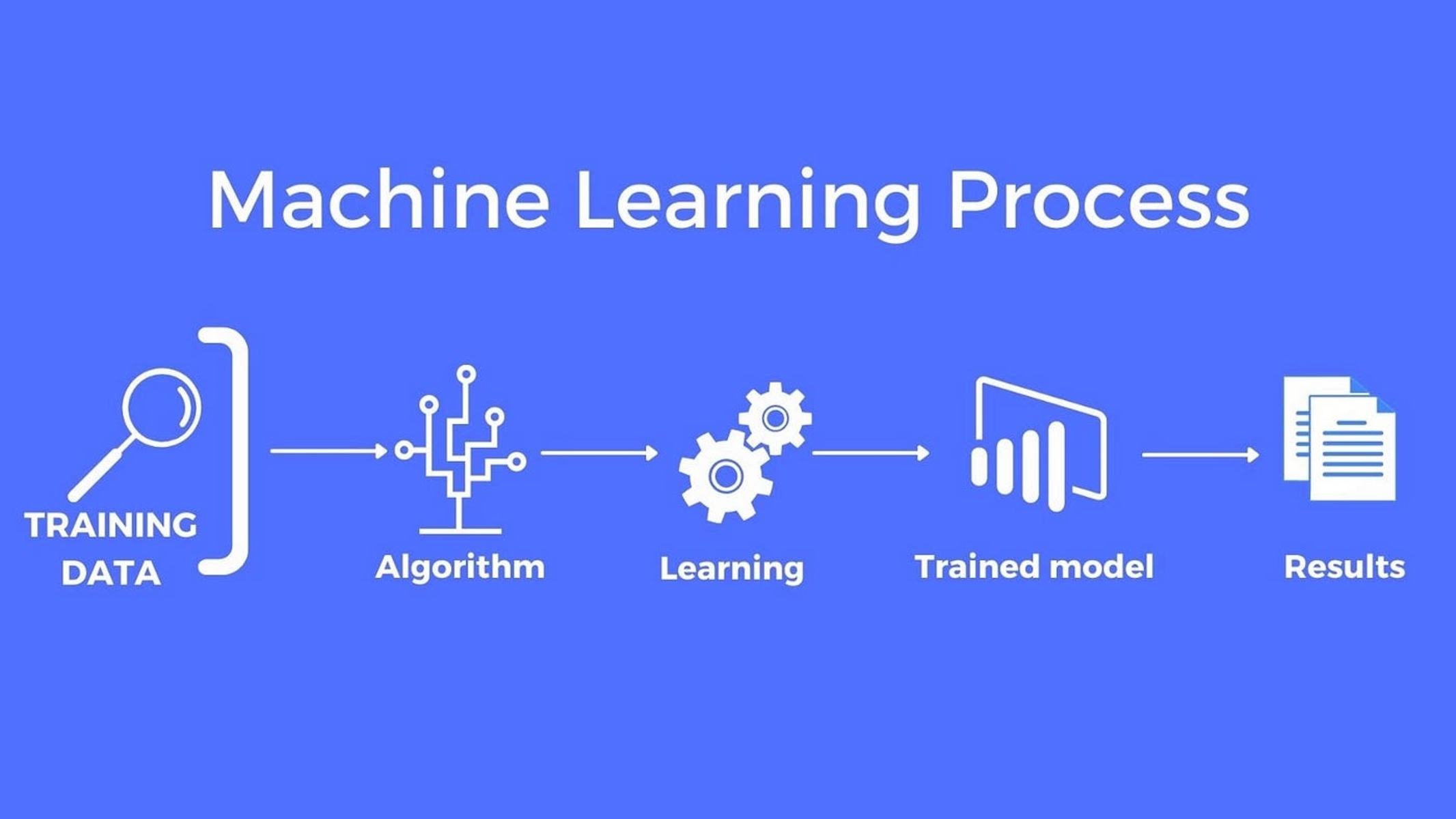
Training the Model

After selecting the appropriate machine learning algorithm, the next step is to train the model using the training set. Training involves fitting the model to the labeled data, allowing it to learn the underlying patterns and relationships between the input features and the target variable. The trained model will then be able to make predictions on new, unseen data.

Let’s explore the general steps involved in training a machine learning model:

1. Prepare the Training Data: Ensure that the training data is properly preprocessed, including handling missing values, encoding categorical variables, and scaling numerical features. The data should be in a format that the chosen algorithm can process.
2. Choose Hyperparameters: Hyperparameters are settings that are not learned by the model during training. They control the behavior and performance of the algorithm. Examples of hyperparameters include learning rate, regularization strength, number of hidden layers in a neural network, or the depth of a decision tree. It is critical to choose appropriate hyperparameters that optimize the model’s performance.
3. Fit the Model: Feed the preprocessed training data into the chosen algorithm and use it to fit the model. This step involves adjusting the model’s internal parameters to minimize the difference between the predicted and actual target values in the training set. The specific fitting process depends on the chosen algorithm.
4. Evaluate the Model: Once the model is trained, it is important to evaluate its performance. Use the evaluation metrics suitable for the specific task to assess how well the model has learned from the training data. Keep in mind that the evaluation should be done on a separate validation or test set, which the model has not seen during training.
5. Iterate and Improve: Based on the evaluation results, you may need to fine-tune the model by adjusting the hyperparameters or trying different algorithms. This iterative process helps improve the model’s performance and generalization capabilities.

Training a machine learning model requires careful tuning and experimentation. It’s essential to strike a balance between underfitting, where the model is too simple and fails to capture the complexity of the data, and overfitting, where the model is too complex and performs poorly on new, unseen data.

By training the model on the training set and iteratively improving its performance, we can develop a robust and accurate model that is capable of making predictions on real-world data. In the next section, we will discuss evaluating the model’s performance and addressing overfitting and underfitting issues.

Evaluating the Model

Once the machine learning model is trained, it is crucial to evaluate its performance to assess its ability to make accurate predictions on new, unseen data. Evaluating the model provides insights into how well it has learned the underlying patterns and allows us to identify any issues or areas for improvement.

Let’s explore some common techniques for evaluating the performance of a machine learning model:

• Accuracy: Accuracy measures the proportion of correctly classified instances. It is a commonly used metric for classification tasks when the classes are balanced. However, accuracy alone may not provide a comprehensive view of the model’s performance, especially when dealing with imbalanced datasets.
• Precision and Recall: Precision and recall are commonly used metrics in binary classification tasks, particularly in cases where one class is of greater importance than the other. Precision measures the proportion of correctly predicted positive cases among the total predicted positive cases, while recall measures the proportion of correctly predicted positive cases among the true positive cases.
• F1-Score: The F1-score is the harmonic mean of precision and recall. It provides a balanced measure of the model’s performance, especially in the presence of class imbalance. It is particularly useful when both precision and recall need to be considered.
• Confusion Matrix: A confusion matrix provides a more detailed evaluation of the model’s performance for multi-class classification tasks. It shows the counts of true positives, true negatives, false positives, and false negatives for each class, enabling a deeper understanding of the model’s predictive abilities.
• Receiver Operating Characteristic (ROC) Curve: The ROC curve is commonly used in binary classification tasks and plots the true positive rate against the false positive rate at different classification thresholds. It provides insights into the trade-off between sensitivity and specificity and helps determine the optimal threshold for decision-making.
• Mean Squared Error (MSE) and Mean Absolute Error (MAE): These metrics are commonly used for regression tasks. MSE calculates the average squared difference between the predicted and actual values, while MAE calculates the average absolute difference. Lower values of these metrics indicate better model performance.

It is important to select the evaluation metrics that are most suitable for the specific machine learning task and domain requirements. It is also important to evaluate the model’s performance on a separate validation set or, ideally, on a completely unseen test set to ensure unbiased evaluation.

By thoroughly evaluating the model’s performance, we gain insights into its strengths and weaknesses. This evaluation helps us understand how well the model generalizes to new data and guides our decision-making for further improvements or model selection.

In the next section, we will discuss techniques for addressing overfitting and underfitting, two common challenges in machine learning.

Handling Overfitting and Underfitting

Overfitting and underfitting are common challenges in machine learning and can both lead to poor model performance. Overfitting occurs when a model learns the training data too well, resulting in poor generalization to new, unseen data. Underfitting, on the other hand, happens when a model is too simple and fails to capture the underlying patterns in the data. It is important to recognize and address these issues to develop a reliable and accurate machine learning model.

Let’s explore some techniques for handling overfitting and underfitting:

• Regularization: Regularization is a technique that introduces a penalty term to the model’s training process, reducing the complexity of the learned function. It helps prevent overfitting by discouraging excessive weight assignment to specific features. Common regularization techniques include L1 regularization (Lasso), L2 regularization (Ridge), and Elastic Net regularization.
• Feature Selection: Overfitting can also occur when the model is trained on irrelevant or redundant features. Feature selection techniques, such as Recursive Feature Elimination (RFE) or selecting the most important features based on feature importance scores, can help mitigate overfitting by selecting only the most informative features.
• Data Augmentation: Data augmentation techniques increase the size and diversity of the training data by applying random transformations or perturbations to the existing samples. By artificially expanding the dataset, data augmentation can help reduce overfitting and improve the model’s ability to generalize to new instances.
• Cross-Validation: Cross-validation is a technique used to estimate the model’s performance on unseen data. It involves splitting the training data into multiple subsets and training the model on each subset while evaluating its performance on the remaining subset. Cross-validation helps assess the model’s ability to generalize and can provide insights into potential overfitting or underfitting.
• Model Ensemble: Ensemble learning involves combining multiple individual models to make predictions. This can be achieved through techniques like bagging (e.g., Random Forest) or boosting (e.g., Gradient Boosting). Ensemble models can help reduce both bias and variance, improving overall model performance and addressing overfitting or underfitting issues.

It is important to strike a balance between model complexity and generalization. A model that is too complex may overfit the training data, resulting in poor performance on unseen data. On the other hand, a model that is too simple may underfit the data and fail to capture the underlying patterns.

Regularization techniques, feature selection, data augmentation, and cross-validation can help mitigate overfitting and underfitting. Model ensemble methods can also be effective in improving model performance and addressing these challenges.

In the next section, we will discuss the process of hyperparameter tuning to optimize the model’s performance.

Hyperparameter Tuning

Hyperparameters are settings or configurations that are not learned by the model during training. They control the behavior and performance of the algorithm. Optimizing these hyperparameters is essential to achieve the best possible performance from a machine learning model. Hyperparameter tuning involves systematically searching for the optimal combination of hyperparameters to maximize the model’s performance.

Let’s explore some techniques for hyperparameter tuning:

• Grid Search: Grid search involves defining a grid of hyperparameter values and exhaustively searching through all possible combinations. It trains and evaluates the model for each combination of hyperparameters and identifies the best performing one based on a specified evaluation metric.
• Random Search: Random search randomly selects combinations of hyperparameter values from predefined ranges. It performs model training and evaluation for each randomly selected combination. Random search is more efficient than grid search when the search space is large.
• Bayesian Optimization: Bayesian optimization is an iterative technique that builds a probability model to approximate the model performance as a function of the hyperparameters. It uses an acquisition function to determine the next set of hyperparameters to evaluate based on the learned probability model. This method can converge to the optimal hyperparameters more efficiently.
• Gradient Descent-Based Optimization: Gradient descent optimization techniques, such as stochastic gradient descent or Adam optimizer, can be used to find optimal hyperparameters for models with differentiable objectives. These techniques involve iteratively updating the hyperparameters based on the gradient information of the evaluation metric.
• Automated Hyperparameter Tuning Libraries: There are also dedicated libraries, such as scikit-optimize, Optuna, or Hyperopt, that provide automated hyperparameter tuning capabilities. These libraries streamline the hyperparameter search process and can handle large search spaces effectively.

During hyperparameter tuning, it is important to establish a meaningful evaluation metric to guide the optimization process. This metric depends on the specific problem at hand, whether it’s accuracy, F1-score, mean squared error, or other appropriate evaluation metrics for the given task.

Hyperparameter tuning is typically performed in conjunction with cross-validation. By using cross-validation, we can estimate the model’s generalization performance for each set of hyperparameters, ensuring that our choice is not biased by the specific validation set used during hyperparameter search.

Remember that hyperparameter tuning can be computationally expensive, especially when the search space is large. It is important to balance optimization time with the available resources and the expected improvement in performance.

By finding the optimal hyperparameters through systematic tuning, we can improve the model’s performance and achieve better predictive accuracy. In the next section, we will explore the process of saving and loading the trained model for future use.

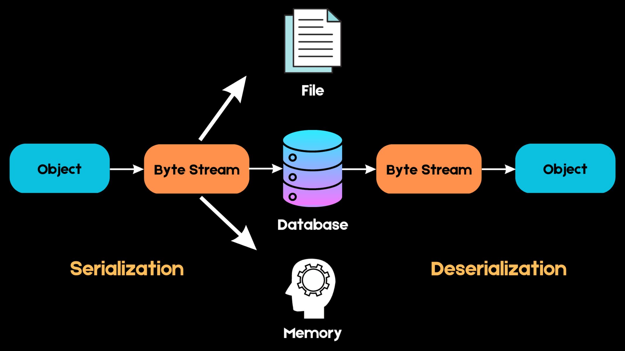
Saving and Loading the Model

Once you have trained a machine learning model and are satisfied with its performance, it is important to save the model’s parameters and structure for future use. Saving the model allows you to quickly deploy it in different environments, make predictions on new data, or share it with others without having to retrain the model from scratch.

Let’s explore how to save and load a trained model in machine learning:

• Serialization: Serialization is the process of converting the model object into a serialized format that can be saved to disk. Most machine learning libraries provide built-in functions or methods to serialize and save the trained model to a file. For example, in scikit-learn, you can use the joblib or pickle module to serialize and save the model.
• Model Format: The serialized model can be saved in various formats, such as pickle (*.pkl) or by using specialized file formats such as HDF5 (*.h5) or ONNX (*.onnx) for interoperability across different machine learning frameworks. Choose the format that best suits your needs in terms of compatibility and ease of use.
• Loading the Model: Loading the model involves deserializing the saved file and recreating the model object in memory. Once the model is loaded, you can make predictions or perform any operations as if you had just trained the model.

Saving the model architecture, trained weights, and other necessary components ensures that you can replicate the model and its functionality accurately, even if the training data or environment changes.

It is important to note that when loading a model, you should verify the compatibility of the model’s saved version and the libraries or dependencies used to load it. Upgrading the libraries or introducing significant changes may result in compatibility issues with the saved model.

You can also incorporate versioning strategies to keep track of various model versions and maintain a history of model improvements or changes.

By saving and loading trained models, you can streamline the deployment process and leverage the model’s capabilities without the need for retraining. This allows for efficient and effective utilization of the trained model in production environments or future projects.

In the next section, we will provide a summary of the key points covered in this article.

Conclusion

In this article, we have explored the process of training a machine learning model in Python. We started by understanding the basics of machine learning and the importance of setting up the environment correctly. We then discussed how to import the necessary libraries, load and prepare the dataset, and perform exploratory data analysis.

We covered techniques for handling missing data and categorical variables, as well as the importance of feature scaling. We also discussed the significance of splitting the dataset into training and test sets to evaluate the model’s performance on unseen data.

Choosing the right machine learning algorithm is crucial, and we explored some common algorithms, including linear regression, logistic regression, decision trees, support vector machines, naive Bayes, and neural networks. We emphasized the importance of evaluating the model’s performance using appropriate evaluation metrics and addressed overfitting and underfitting issues.

Hyperparameter tuning was discussed as a way to optimize the model’s performance, and we explored techniques such as grid search, random search, Bayesian optimization, and gradient descent-based optimization. Finally, we highlighted the importance of saving and loading the trained model to enable its deployment and use in different environments.

By following these steps and practices, you can develop reliable and accurate machine learning models that can make informed predictions and decisions based on data. Remember to constantly iterate and improve your model by fine-tuning hyperparameters, refining feature selection, and exploring new techniques as the field of machine learning continues to evolve.

With the knowledge gained from this article, you have the foundation to embark on your journey as a skilled practitioner in training machine learning models in Python. Good luck with your future projects and the incredible opportunities that lie ahead in the field of machine learning!