Introduction
Gaussian distribution, also known as the normal distribution or the bell curve, is a fundamental concept in statistics and probability theory. It is widely used in various fields, including machine learning. Understanding Gaussian distribution is crucial for developing and evaluating machine learning models that rely on probabilistic assumptions.
At its core, Gaussian distribution describes the probability distribution of a random variable. It is characterized by its symmetric bell-shaped curve, with the majority of values clustering around the mean. The distribution is fully defined by two parameters: the mean and the variance.
In machine learning, Gaussian distribution plays a significant role in modeling and predicting continuous variables. Many algorithms, such as linear regression and Gaussian mixture models, assume that the underlying data follows a Gaussian distribution. By leveraging this assumption, machine learning models can estimate the most likely values and make accurate predictions.
One of the key properties of the Gaussian distribution is the Central Limit Theorem. This theorem states that the sum or average of a large number of independent and identically distributed random variables will have an approximately Gaussian distribution, regardless of the original distribution of the variables. This property makes Gaussian distribution a powerful tool in statistical inference and hypothesis testing.
In this article, we will delve deeper into the concept of Gaussian distribution and explore its properties, including the probability density function, mean, and variance. We will also discuss the standard normal distribution and how it relates to Gaussian distribution. Additionally, we will highlight the application of Gaussian distribution in machine learning and its importance in various algorithms and models.
By understanding and harnessing the power of Gaussian distribution, machine learning practitioners can make more informed decisions, improve model performance, and gain valuable insights from their data.
What is Gaussian Distribution?
Gaussian distribution, also known as the normal distribution or bell curve, is a continuous probability distribution that describes the random variable’s probability density function. It is characterized by its bell-shaped curve, with the highest point at the mean and symmetric tails on either side.
The key defining feature of Gaussian distribution is that it is fully determined by two parameters: the mean (μ) and the variance (σ^2). The mean represents the center of the distribution, while the variance controls the spread or dispersion of the data. The standard deviation (σ) is the square root of the variance and provides a measure of the average deviation from the mean.
The probability density function (PDF) of a Gaussian distribution is given by:
f(x) = (1 / √(2πσ^2)) * e^(-(x-μ)^2 / (2σ^2))
where x is the random variable, e is the base of the natural logarithm, and π is a mathematical constant approximately equal to 3.14159.
Gaussian distribution exhibits several important properties that make it widely used in statistical analysis and modeling. One such property is that it is symmetric around the mean, meaning that the probability of observing a value to the left or right of the mean is equal. This symmetry helps in making predictions and calculating probabilities.
Another property is that many real-world phenomena naturally follow a Gaussian distribution. Examples include physical measurements like human height and weight, test scores, and errors in measurements. Gaussian distribution also emerges as an approximation in cases where the Central Limit Theorem applies.
In summary, Gaussian distribution is a fundamental concept in statistics and probability theory. It is characterized by its bell-shaped curve, with the mean and variance serving as key parameters. Understanding Gaussian distribution is crucial for various statistical analyses and machine learning algorithms that rely on probabilistic assumptions to model and predict data.
Properties of Gaussian Distribution
Gaussian distribution, also known as the normal distribution, exhibits several important properties that make it a fundamental concept in statistics and probability theory. Understanding these properties is essential for accurately modeling and analyzing data using Gaussian distribution.
1. Symmetry: One of the key properties of Gaussian distribution is its symmetry. The curve of the distribution is perfectly symmetric around the mean, which means that the probability of observing a value to the left or right of the mean is equal. This symmetry makes Gaussian distribution a useful tool for making predictions and calculating probabilities.
2. Bell-shaped Curve: Another property of Gaussian distribution is its characteristic bell-shaped curve. The majority of values cluster around the mean, and the probability decreases as the values move away from the mean in either direction. This shape is a result of the exponential term in the probability density function, which tapers off the probabilities as the values move further from the mean.
3. Mean and Variance: The mean (μ) and variance (σ^2) are the two key parameters of Gaussian distribution. The mean represents the center of the distribution and indicates the expected value of the random variable. The variance determines the spread or dispersion of the data around the mean. It measures the average squared deviation of the values from the mean. The standard deviation (σ) is the square root of the variance and provides a measure of the average deviation from the mean.
4. Central Limit Theorem: The Central Limit Theorem is a significant property related to Gaussian distribution. It states that the sum or average of a large number of independent and identically distributed random variables will have an approximately Gaussian distribution, regardless of the original distribution of the variables. This property makes Gaussian distribution a powerful tool in statistical inference and hypothesis testing.
5. Normality Assumption: Many statistical methods and machine learning algorithms assume that the underlying data follows a Gaussian distribution. This normality assumption simplifies the analysis and allows for the application of various statistical techniques. However, it is essential to validate this assumption for the data at hand before relying exclusively on Gaussian distribution in modeling and analysis.
Gaussian distribution exhibits these properties, making it a versatile and widely used tool in statistics and machine learning. By understanding and leveraging these properties, practitioners can accurately model data, make predictions, and derive meaningful insights from their analyses.
The Probability Density Function (PDF)
The Probability Density Function (PDF) is a fundamental concept in Gaussian distribution. It describes the probability distribution of a continuous random variable. For a Gaussian distribution, the PDF is given by the following equation:
f(x) = (1 / √(2πσ^2)) * e^(-(x-μ)^2 / (2σ^2))
In this equation, x represents the random variable, μ is the mean, and σ is the standard deviation.
The PDF provides a way to calculate the probability that the random variable x will fall within a certain range. Since Gaussian distribution is continuous, the probability of obtaining an exact value for x is zero. Instead, the PDF gives us the relative likelihood of obtaining values within a specific range.
The PDF of a Gaussian distribution has several important properties:
1. Area under the Curve: The integral of the PDF over its entire range is equal to 1. This means that the total probability of all possible values for the random variable is equal to 1.
2. Symmetry: The PDF is symmetric around the mean μ. The probability is highest at the mean and decreases symmetrically as the values move away from the mean in either direction.
3. Inflection Points: The points where the PDF changes from concave up to concave down, or vice versa, are called inflection points. These points occur at x = μ ± σ, and they mark the points where the curvature of the PDF changes.
4. Tail Behavior: As the values move further from the mean, the probability density decreases exponentially. However, it never reaches zero, meaning there is always a non-zero probability of obtaining extreme values.
The PDF of Gaussian distribution is a fundamental tool in analyzing and modeling data. It allows us to calculate probabilities, estimate the likelihood of obtaining values within a specific range, and understand the shape and characteristics of the distribution. By utilizing the PDF, practitioners can make informed decisions, develop accurate models, and gain valuable insights from their data.
Mean and Variance
The mean and variance are essential parameters that characterize Gaussian distribution and provide valuable insights into the data. Understanding these parameters is crucial for interpreting the distribution and making predictions based on it.
Mean (μ): The mean of a Gaussian distribution represents the central tendency or average value of the data. It is denoted by the symbol μ. In the context of the PDF, the mean corresponds to the peak or highest point on the distribution curve. It indicates the most likely or expected value of the random variable.
The mean of a Gaussian distribution can be calculated using the following formula:
μ = ∑(xi) / n
where xi represents the individual values of the random variable and n is the total number of values.
Variance (σ^2): The variance measures the dispersion or spread of the data around the mean. It quantifies how much the values deviate from the mean. A higher variance indicates a wider spread of the data, while a lower variance implies a narrower range. The variance is denoted by the symbol σ^2.
The variance of a Gaussian distribution can be calculated using the following formula:
σ^2 = (∑(xi – μ)^2) / n
where xi represents the individual values of the random variable, μ is the mean, and n is the total number of values.
The standard deviation (σ) is the square root of the variance and provides a measure of the average deviation from the mean. It is commonly used to describe the spread of the data in Gaussian distribution.
The mean and variance are important parameters that allow us to understand the central tendency and spread of the data in a Gaussian distribution. By analyzing these parameters, we can gain insights into the characteristics of the distribution and make predictions based on its properties.
Standard Normal Distribution
In statistics, the standard normal distribution, also known as the Z-distribution or the standard Gaussian distribution, holds a special place due to its standardized form. It is a specific instance of the Gaussian distribution with a mean of 0 and a standard deviation of 1. The standard normal distribution is widely used in statistical analysis and hypothesis testing.
The probability density function (PDF) of the standard normal distribution is given by:
f(x) = (1 / √(2π)) * e^(-x^2 / 2)
Here, x represents the random variable. The PDF describes the relative likelihood of observing different values of x within the standard normal distribution.
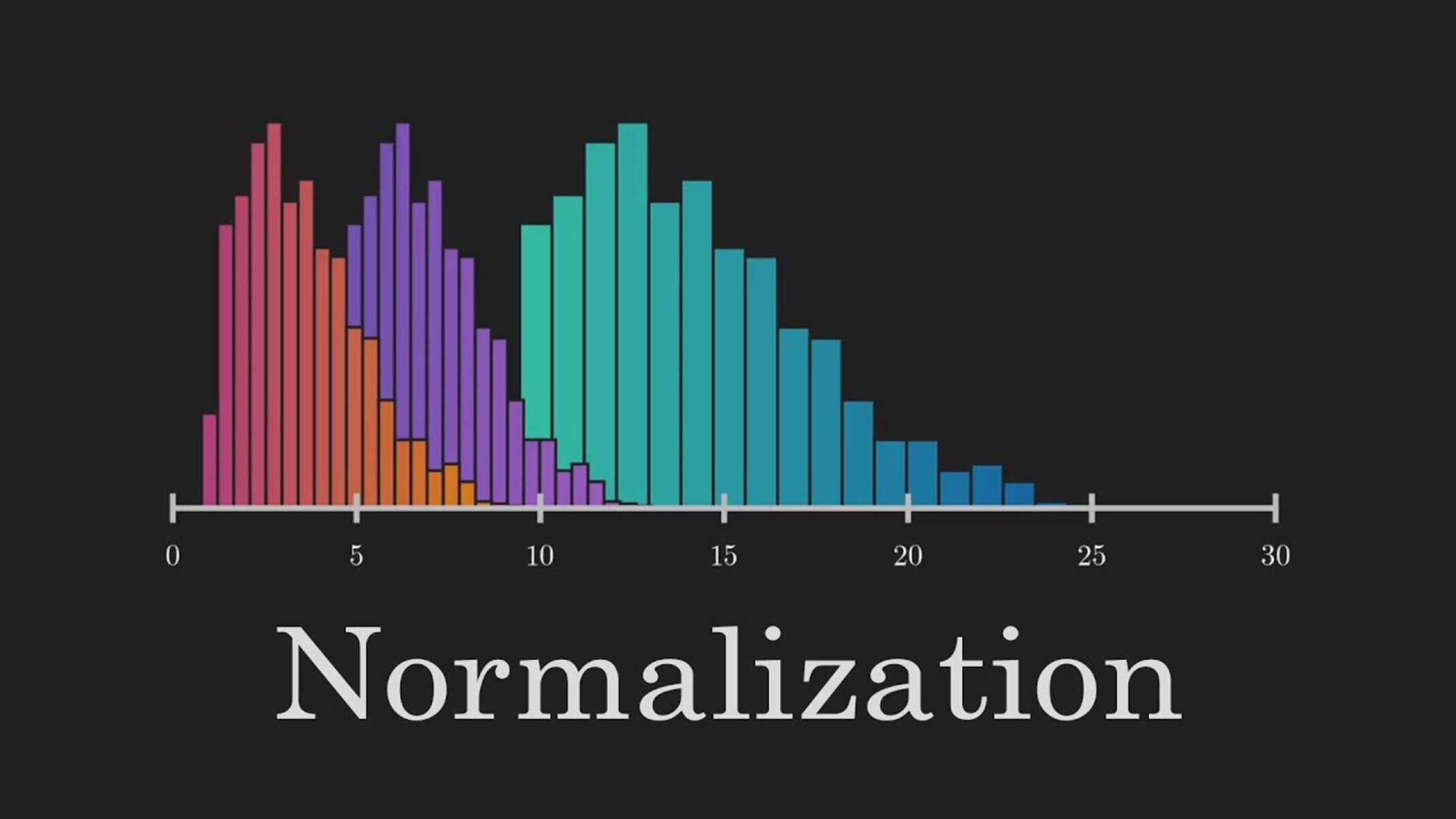
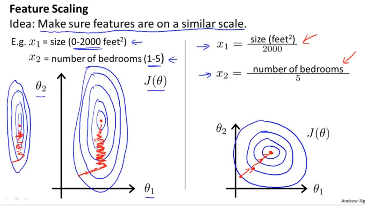
The standard normal distribution is particularly valuable because it allows us to convert any Gaussian distribution to the standard form. This transformation is known as standardization or normalization. By standardizing the data, we can compare different Gaussian distributions and determine how likely a value is relative to the mean.
The process of standardization involves subtracting the mean and dividing by the standard deviation. This yields a Z-score, representing the number of standard deviations by which a particular value deviates from the mean. The formula to calculate the Z-score is as follows:
Z = (x – μ) / σ
Here, x represents an individual value, μ is the mean, and σ is the standard deviation.
The Z-score allows us to determine the relative position of a value within a Gaussian distribution. A positive Z-score indicates that a value is above the mean, while a negative Z-score indicates it is below the mean. Additionally, we can use Z-scores to calculate percentiles and determine the proportion of values below or above a given threshold.
The standard normal distribution serves as a reference for statistical analyses. By standardizing data to the standard normal distribution, we can easily compare different datasets or calculate probabilities and percentiles. It provides a standardized framework for data analysis, hypothesis testing, and making statistical inferences.
Z-Scores and Percentiles
Z-scores and percentiles play a crucial role in understanding and analyzing Gaussian distributions. They provide a standardized method for comparing data points, determining their relative positions, and calculating probabilities.
A Z-score, also known as a standard score, measures the number of standard deviations a particular value is from the mean in a Gaussian distribution. It is calculated using the formula:
Z = (x – μ) / σ
Here, x represents an individual value, μ is the mean, and σ is the standard deviation. A positive Z-score indicates a value above the mean, while a negative Z-score indicates a value below the mean.
Z-scores allow us to determine the relative position of a value within a Gaussian distribution. For example, a Z-score of 2 means that the value is two standard deviations above the mean. Z-scores can be used to identify outliers, compare data points across different distributions, and calculate probabilities.
Percentiles, on the other hand, provide a way to determine the position of a value within a distribution relative to all other values. The percentile rank of a value represents the percentage of values in the distribution that are below that value.
For example, if a value has a percentile rank of 80, it means that 80% of the values in the distribution are below that value. Similarly, a percentile rank of 50 represents the median, indicating that 50% of the values are below and 50% are above that value.
Percentiles are useful for understanding the spread of data and identifying extremes. For instance, the 95th percentile represents a value that is greater than 95% of the values in the distribution.
In Gaussian distributions, the Z-score and percentile rank are related. Z-scores can be converted to percentiles using a Z-score table or statistical software. This conversion allows us to determine the percentage of observations within a specific range or above a certain threshold.
Z-scores and percentiles are essential tools for analyzing Gaussian distributions. They provide a standardized way to compare values, calculate probabilities, and understand the position of a value within a distribution. By utilizing these measures, we can make meaningful inferences and draw valuable insights from the data.
Application of Gaussian Distribution in Machine Learning
Gaussian distribution, with its well-defined properties and probabilistic nature, finds extensive applications in machine learning algorithms and models. By leveraging the assumptions of Gaussian distribution, practitioners can develop powerful predictive models and make accurate probabilistic predictions.
1. Linear Regression: Gaussian distribution plays a fundamental role in linear regression models. The linear regression assumes that the relationship between the independent variables and the dependent variable is linear and that the errors are normally distributed with constant variance. By assuming the errors to follow a Gaussian distribution, the maximum likelihood estimation technique can be used to estimate the model parameters and make predictions.
2. Gaussian Mixture Models: Gaussian mixture models (GMMs) are widely used for density estimation and clustering tasks. A GMM assumes that the data is generated from a mixture of Gaussian distributions. It uses the expectation-maximization algorithm to estimate the parameters of the individual Gaussian components, such as means, variances, and weights. GMMs can handle complex data distributions and are often used for image segmentation, anomaly detection, and clustering.
3. Bayesian Inference: Bayesian inference is a probabilistic approach that involves updating prior beliefs based on observed data. In many cases, the prior and posterior distributions in Bayesian inference are assumed to be Gaussian. This assumption simplifies the mathematical calculations and allows for the use of conjugate priors, which lead to closed-form solutions. Gaussian distributions also play a crucial role in variational inference and Markov Chain Monte Carlo (MCMC) methods.
4. Anomaly Detection: Anomaly detection is the task of identifying rare and unusual instances in a dataset. Gaussian distribution is often used as a basis for detecting anomalies. By modeling the normal behavior of the data using Gaussian distribution, any significant deviation from the expected pattern can be flagged as an anomaly. This approach is commonly used in fraud detection, intrusion detection, and system monitoring.
5. Naive Bayes Classifier: Naive Bayes is a simple yet powerful probabilistic classifier. It assumes that the features are conditionally independent given the class labels. When the features are continuous, a common approach is to assume that they follow a Gaussian distribution. This assumption allows for the use of the Gaussian Naive Bayes classifier, which can handle continuous data and make classification predictions based on the probability distributions of the features.
Gaussian distribution provides a solid foundation for various machine learning algorithms. Its probabilistic nature allows for uncertainty modeling, accurate prediction, and statistical inference. By making appropriate assumptions and leveraging the properties of Gaussian distribution, practitioners can build robust, interpretable, and effective machine learning models for a wide range of applications.
Conclusion
Gaussian distribution, with its bell-shaped curve and well-defined properties, is a fundamental concept in statistics and probability theory. It finds wide applications in various fields, including machine learning. Understanding Gaussian distribution is crucial for developing and evaluating machine learning models that rely on probabilistic assumptions.
In this article, we have explored the concept of Gaussian distribution and its properties. We have discussed the probability density function (PDF), mean, and variance, which are key components of Gaussian distribution. Additionally, we have examined the standard normal distribution and its significance in statistical analysis.
We have also highlighted the application of Gaussian distribution in machine learning. From linear regression to Gaussian mixture models, Gaussian distribution plays a significant role in modeling and predicting continuous variables. Its assumptions are leveraged in Bayesian inference, anomaly detection, and Naive Bayes classification, among other applications.
By understanding and effectively utilizing Gaussian distribution, machine learning practitioners can build more accurate and robust models. Gaussian distribution provides a solid foundation for handling uncertainty, making predictions, and quantifying the likelihood of events.
However, it is important to note that Gaussian distribution is not always the appropriate model for every dataset. It is necessary to assess the data and validate the assumptions before relying solely on Gaussian distribution. Additionally, other probability distributions, such as exponential or binomial distributions, may better suit specific datasets and modeling requirements.
In conclusion, Gaussian distribution serves as a powerful tool in machine learning, allowing practitioners to make informed decisions, improve model performance, and gain valuable insights from their data. By understanding its properties and applications, machine learning practitioners can harness the full potential of Gaussian distribution and enhance their predictive modeling capabilities.


