Introduction
Welcome to the world of machine learning! As technology advances, machine learning has become an integral part of many industries, revolutionizing the way we make decisions and automate processes. However, one of the key challenges in machine learning is improving the accuracy of our models.
Having an accurate machine learning model is crucial because it directly impacts the effectiveness and reliability of the predictions and decisions made based on the model’s output. Inaccurate models can lead to poor business outcomes, incorrect predictions, and wasted resources.
In this article, we will explore various steps that can help improve the accuracy of a machine learning model. From collecting and cleaning the data to hyperparameter tuning and ensembling models, we will cover the essential techniques and strategies that can significantly enhance the performance of your models.
Each step in the process plays a vital role in refining the model’s accuracy and ensuring it delivers reliable results. By following these steps, you will be better equipped to build robust and accurate machine learning models that can drive actionable insights and enable smarter decision-making.
Throughout this article, we will dive into the practical aspects of each step and provide valuable insights and tips that you can implement in your machine learning projects. Whether you are a beginner or an experienced practitioner, these techniques will empower you to take your models to the next level.
So, if you are ready to elevate the accuracy of your machine learning models, let’s get started with the first step – collecting and cleaning the data.
Step 1: Collecting and Cleaning the Data
The first step towards improving the accuracy of a machine learning model is to collect and clean the data. High-quality and well-prepared data is the foundation for building accurate models that can make reliable predictions.
When collecting the data, it is important to ensure that the dataset is representative of the problem you are trying to solve. Bias in the data can lead to biased predictions, so it is crucial to include diverse samples that cover various scenarios and edge cases.
Once the data is collected, the next step is to clean it. Cleaning the data involves removing any inconsistencies, errors, or outliers that can negatively impact the model’s performance. Missing values need to be handled appropriately by either imputing them or removing the corresponding samples if the missing data is substantial.
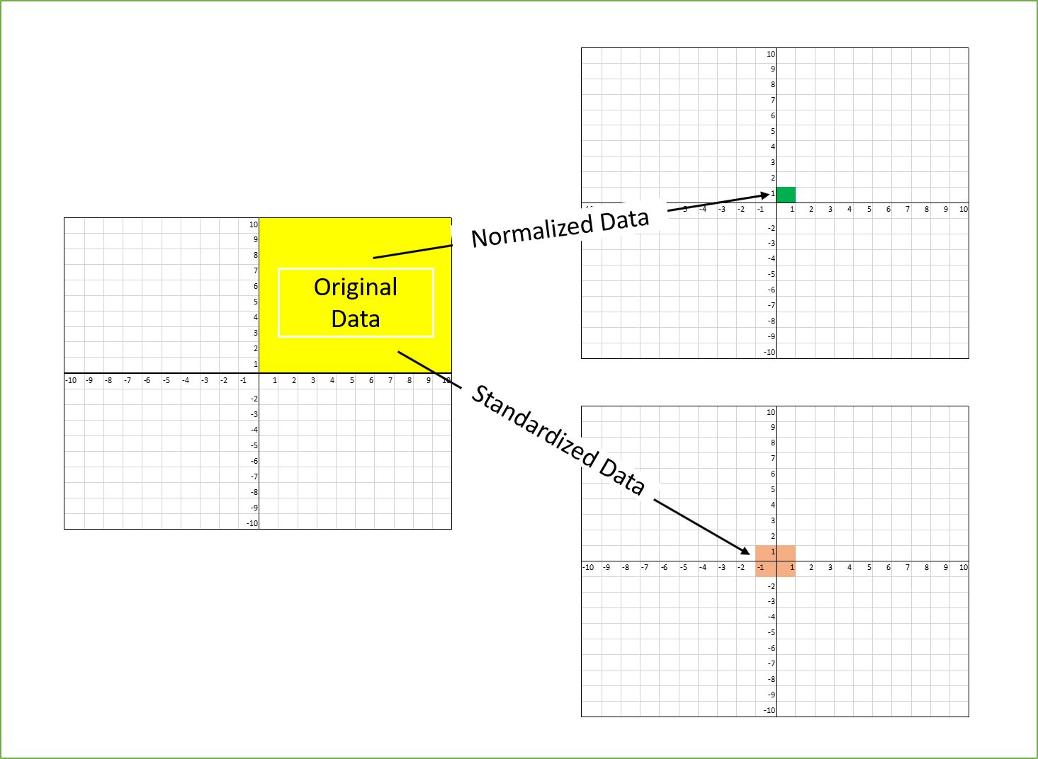
Feature scaling is another important aspect of data cleaning. Scaling the features helps to bring them to a similar range and prevent certain features from dominating the model’s training process. Common scaling techniques include normalization and standardization.
In addition, categorical variables need to be encoded properly to make them suitable for machine learning algorithms. This can be achieved through one-hot encoding or label encoding, depending on the nature of the categorical data.
Another crucial consideration is handling imbalanced data. In many real-world scenarios, datasets may have imbalances in class distribution, leading to biased models. Techniques such as oversampling and undersampling can help address this issue and ensure that the model learns from all classes equally.
Finally, it is important to split the dataset into training and testing sets. The training set is used to train the model, while the testing set is used to evaluate its performance. This split ensures that the model’s accuracy is assessed on unseen data, giving a realistic estimate of its performance in real-world scenarios.
By diligently collecting and cleaning the data, you lay the groundwork for building accurate machine learning models. The quality and cleanliness of the data directly impact the model’s ability to uncover meaningful patterns and make accurate predictions.
In the next step, we will delve into exploratory data analysis, where we visualize and analyze the data to gain insights and further refine our models. So, let’s move on to step 2!
Step 2: Exploratory Data Analysis
Exploratory Data Analysis (EDA) is a vital step in the machine learning process. It involves visualizing and analyzing the data to gain insights and better understand its characteristics.
EDA helps us uncover patterns, relationships, and outliers in the data, which can guide us in making informed decisions during the model-building process.
One of the first steps in EDA is to visualize the data using various charts and graphs. Histograms can provide insights into the distribution of numerical features, helping us understand the range and spread of the data. Scatter plots enable us to identify relationships between different features, aiding in feature selection and engineering.
Box plots are useful for detecting outliers, which are data points that significantly deviate from the rest of the distribution. Outliers can have a significant impact on the model’s performance, and it is essential to handle them appropriately, either by removing them or applying appropriate transformations to mitigate their effects.
Correlation analysis is another crucial aspect of EDA. By calculating correlation coefficients, we can understand the strength and direction of the relationships between variables. Highly correlated variables may indicate redundancy, and feature selection techniques such as dimensionality reduction can be applied to remove unnecessary variables.
EDA also involves examining the target variable (dependent variable). Understanding the distribution of the target variable can help us determine the appropriate algorithm and evaluation metrics for our model. For example, if the target variable is imbalanced, techniques like oversampling, undersampling, or using evaluation metrics like precision and recall become necessary.
Moreover, EDA allows us to identify missing or inconsistent data. Addressing these issues before training our model ensures that we are working with the most accurate and complete dataset.
As we analyze the data, we might come across interesting insights or patterns that can suggest additional features or transformations to improve our model’s accuracy. EDA is an iterative process that helps us refine our understanding of the data and optimize our feature engineering techniques.
By conducting a thorough exploratory data analysis, we gain valuable insights into our dataset, enabling us to make informed decisions in the subsequent steps of the machine learning pipeline. The information obtained through EDA guides the feature engineering process and influences the choice of algorithms and hyperparameter tuning strategies.
Now that we have explored the data, it’s time to move on to step 3: feature engineering. Stay tuned!
Step 3: Feature Engineering
Feature engineering is a crucial step in improving the accuracy of a machine learning model. It involves creating new features or transforming existing ones to enhance the information available to the model and make it more effective in capturing patterns and relationships within the data.
Feature engineering is a creative process that requires deep domain knowledge and a thorough understanding of the dataset. It involves selecting, combining, and transforming features to extract the most relevant information and represent it in a way that is meaningful to the model.
One common technique in feature engineering is scaling or normalizing numerical features. Scaling ensures that different features, which may have different scales and units, are put on a similar scale. This prevents certain features from dominating the learning process and allows the model to effectively learn from all features.
In addition to scaling, feature engineering may involve creating interaction terms or polynomial features to capture non-linear relationships between variables. This can be done by multiplying or combining relevant features to create new ones.
Another important aspect of feature engineering is handling categorical variables. Categorical variables need to be converted into numerical form for most machine learning algorithms to process them. This can be achieved through techniques like one-hot encoding (representing each category as a binary feature) or label encoding (assigning unique integers to each category).
Domain-specific knowledge plays a significant role in feature engineering. It helps identify and engineer domain-specific features that can have a strong impact on model performance. For example, in natural language processing, features like word frequency, n-grams, or sentiment scores can be engineered to improve text classification models.
During feature engineering, it is important to keep the dimensionality of the dataset in check. High-dimensional datasets can lead to overfitting and increased computational complexity. Techniques such as dimensionality reduction (e.g., principal component analysis or feature selection) can be used to select the most relevant features or create new feature representations that capture the most important information.
By carefully engineering features, we provide our model with the necessary information to make accurate predictions. Feature engineering is a continuous process that involves iterations and fine-tuning throughout the machine learning pipeline. It is an art that combines creativity, domain knowledge, and data understanding to extract the maximum predictive power from the dataset.
Now that we have enhanced our feature set, let’s move on to step 4: choosing the right algorithm for our model. Stay tuned!
Step 4: Choosing the Right Algorithm
Choosing the right algorithm is a critical step in improving the accuracy of a machine learning model. The algorithm determines how the model learns from the data and makes predictions. Different algorithms have different strengths and weaknesses, and selecting the appropriate one can significantly impact the model’s performance.
When choosing an algorithm, it is essential to consider the nature of the problem, the type and size of the dataset, and the available computational resources. Understanding the characteristics of the data and the requirements of the problem will guide us in selecting the most suitable algorithm.
For example, if the problem is a classification task with a small dataset, algorithms like Logistic Regression, Naive Bayes, or Support Vector Machines (SVM) may be effective. These algorithms work well with limited data and can handle binary or multi-class classification problems.
For problems involving large datasets or high-dimensional data, algorithms like Random Forests, Gradient Boosting Machines (GBM), or Deep Learning Neural Networks (using frameworks like TensorFlow or Keras) might be appropriate. These algorithms have the ability to handle complex relationships and capture intricate patterns in the data.
If the problem involves regression, algorithms like Linear Regression, Decision Trees, or Ensemble methods such as Bagging or Boosting (e.g., AdaBoost, XGBoost) can be considered for accurate predictions of continuous variables.
It is also worth considering algorithmic advancements specific to the problem domain. For example, if the problem involves image classification, deep learning algorithms like Convolutional Neural Networks (CNNs) have proven to be highly effective in recent years.
Choosing the right algorithm may require experimentation and comparison. It is often useful to try multiple algorithms and evaluate their performance using appropriate evaluation metrics. Cross-validation techniques can help assess the robustness and generalization capabilities of the models.
Furthermore, optimizing hyperparameters for the chosen algorithm can significantly improve its accuracy. Hyperparameters are adjustable settings that control the learning process of the algorithm. Techniques like grid search or random search can be used to find the best combination of hyperparameters that yield the highest accuracy.
By carefully selecting the appropriate algorithm for our specific problem and dataset, we can leverage its strengths and maximize the accuracy of our model. The chosen algorithm acts as the backbone of the model, enabling it to learn from the data and make accurate predictions.
Now that we have chosen our algorithm, let’s move on to step 5: training the model using our prepared dataset. Stay tuned!
Step 5: Training the Model
Once we have collected and cleaned our data, performed exploratory data analysis, engineered relevant features, and selected the appropriate algorithm, we are ready to move on to the next critical step: training the model.
Training the model involves feeding our prepared dataset into the selected algorithm and allowing it to learn from the data. During this process, the model adjusts its internal parameters based on the patterns and relationships it discovers in the training data.
The training process typically involves iteratively updating the model’s parameters to minimize a predefined loss function. The loss function measures the discrepancy between the model’s predictions and the actual values in the training data.
The choice of loss function depends on the type of problem we are trying to solve. For regression tasks, common loss functions include Mean Squared Error (MSE) or Root Mean Squared Error (RMSE). For classification tasks, Cross-Entropy Loss or Log Loss may be used.
During training, it is important to split the data into training and validation sets. The training set is used to update the model’s parameters, while the validation set helps us monitor the model’s performance on unseen data and detect any signs of overfitting.
Overfitting occurs when the model becomes too complex and starts to memorize the training examples, performing poorly on new, unseen data. Techniques such as early stopping and regularization can be employed to mitigate overfitting and improve generalization.
Training a model involves finding a balance between underfitting and overfitting. Underfitting occurs when the model is too simple to capture the underlying patterns in the data, resulting in poor performance. Regular model evaluation during the training process helps us identify these issues and make necessary adjustments.
Once the model has been trained, it can be saved and used for making predictions on new, unseen data. The accuracy and reliability of these predictions depend on the training process and the quality of the data used.
It is important to note that training a model may require significant computational resources and time, especially for complex algorithms or large datasets. Therefore, it is crucial to optimize the training process, choose appropriate batch sizes, and adjust other hyperparameters to ensure efficient training.
By effectively training the model, we enable it to learn from the data and capture the underlying patterns and relationships. The success of our trained model depends on the accuracy of the training process and the suitability of the chosen algorithm for the problem at hand.
With our model trained, we can now proceed to step 6: evaluating its performance to determine how well it can generalize to new, unseen data.
Step 6: Evaluating Model Performance
Once our model has been trained, it is crucial to evaluate its performance to ensure its accuracy and reliability in making predictions on new, unseen data. Evaluating the model’s performance helps us assess its ability to generalize and make accurate predictions in real-world scenarios.
There are various evaluation metrics that can be used, depending on the nature of the problem. For classification tasks, metrics such as accuracy, precision, recall, and F1 score can be employed. These metrics provide insights into the model’s ability to correctly classify different classes and handle imbalanced data.
For regression tasks, evaluation metrics like Mean Absolute Error (MAE), Mean Squared Error (MSE), and Root Mean Squared Error (RMSE) can be useful in assessing the model’s accuracy in predicting continuous variables.
When evaluating the model, it is important to use evaluation techniques that provide an unbiased estimate of its performance. Cross-validation is a widely used technique that helps us assess the model’s robustness and generalization capabilities. It involves splitting the data into multiple subsets and training and evaluating the model on different combinations of these subsets.
Evaluating the model’s performance on a separate testing set is also crucial, as it measures its accuracy on unseen data. This testing set should not have been used during the training process, ensuring a fair evaluation.
Model performance can also be visualized using various techniques. For classification tasks, a confusion matrix can provide insights into the model’s performance on different classes. ROC curves and Precision-Recall curves can help us understand the trade-offs between true positive rate and false positive rate.
Additionally, learning curves can be plotted to visualize the model’s convergence and detect issues like underfitting or overfitting. These curves show how the model’s performance changes as the amount of training data increases.
By rigorously evaluating the model’s performance using appropriate metrics and techniques, we gain a clear understanding of its strengths and weaknesses. This evaluation helps us make informed decisions about our model and identify areas for improvement.
If the model’s performance is not satisfactory, it may be necessary to revisit previous steps such as feature engineering, hyperparameter tuning, or even collecting additional data. Iterative refinement and fine-tuning based on evaluation results are often necessary to improve the model’s accuracy and reliability.
Once we are satisfied with the model’s performance, we can proceed to the next step: hyperparameter tuning. By tuning the model’s hyperparameters, we can further enhance its performance and maximize its accuracy.
Step 7: Hyperparameter Tuning
Hyperparameter tuning is a crucial step in optimizing the performance of a machine learning model. Hyperparameters are adjustable parameters that define the behavior and flexibility of the model, such as learning rate, regularization strength, or the number of hidden layers in a neural network.
The default values or initial choices of hyperparameters may not be optimal for every model and dataset. Hyperparameter tuning involves finding the best combination of hyperparameters that yield the highest performance and accuracy for our specific problem.
There are various techniques for hyperparameter tuning, one of which is grid search. Grid search involves defining a range of possible values for each hyperparameter and systematically trying out all combinations to find the best set of hyperparameters.
Another technique is random search, where hyperparameters are randomly sampled from predefined ranges. This approach can be more efficient than grid search, especially when the hyperparameter space is large.
Cross-validation is often used during hyperparameter tuning to evaluate the performance of each set of hyperparameters. By using a subset of training data for validation, we can estimate how well the model will generalize to unseen data when using the selected hyperparameters.
During hyperparameter tuning, it is important to strike a balance between model complexity and performance. Overly complex models may lead to overfitting on the training data, resulting in poor generalization. On the other hand, overly simplified models may underfit the data and fail to capture meaningful patterns.
Hyperparameter tuning can be computationally expensive, especially for complex models or large datasets. Techniques like Bayesian optimization or evolutionary algorithms can help streamline the search process and find optimal hyperparameters more efficiently.
By carefully tuning the model’s hyperparameters, we optimize its performance and accuracy, ensuring it achieves the best possible predictions. Hyperparameter tuning is an iterative process, and as we make further improvements to the model, we may need to revisit hyperparameter tuning to fine-tune its performance.
Once we have identified the best set of hyperparameters, it is time to move on to step 8: handling overfitting. Overfitting occurs when the model becomes too complex and performs well on the training data but fails to generalize to new, unseen data. Handling overfitting is crucial for building a reliable and accurate machine learning model.
Step 8: Handling Overfitting
Handling overfitting is a critical step in improving the accuracy and generalization capabilities of a machine learning model. Overfitting occurs when the model becomes too complex or does not have enough data to learn from, causing it to memorize the training examples rather than capturing the underlying patterns.
There are several techniques that can be employed to address overfitting and improve the model’s performance:
1. Regularization: Regularization is a technique that introduces a penalty term to the loss function during training. It helps prevent the model from becoming overly complex by adding constraints on the model parameters. Common regularization techniques include L1 and L2 regularization.
2. Dropout: Dropout is a regularization technique specific to neural networks. It randomly sets a fraction of the neurons to zero during training, preventing them from being overly dependent on a specific subset of features. Dropout acts as a form of ensemble learning, making the model more resilient to overfitting.
3. Early stopping: Early stopping involves monitoring the performance of the model on a validation set during training. If the validation performance starts to deteriorate after an initial improvement, training is stopped early to prevent further overfitting. This technique ensures that the model is trained for the optimal number of iterations.
4. Feature selection: Feature selection involves choosing the most relevant features from the dataset. Removing irrelevant or redundant features reduces the complexity of the model and prevents it from overfitting on noise or uninformative features. Techniques like backward elimination or forward selection can be used for feature selection.
5. Cross-validation: Cross-validation allows us to assess the performance of the model on multiple subsets of the data. It provides a more robust evaluation by averaging the results across different partitions of the data. By using cross-validation, we can detect overfitting and make adjustments to the model accordingly.
6. Data augmentation: Data augmentation techniques involve generating synthetic data from the existing dataset. By applying transformations or introducing slight variations to the existing samples, we can increase the diversity of the training data, reducing the risk of overfitting. Data augmentation is particularly useful in computer vision or natural language processing tasks.
By applying these techniques, we can mitigate overfitting and improve the model’s generalization capabilities. It is important to strike a balance between model complexity and performance, ensuring that the model learns meaningful patterns without memorizing the training data.
Handling overfitting is an iterative process, and it may require revisiting previous steps such as feature engineering or hyperparameter tuning. Continuously monitoring the model’s performance and making necessary adjustments will lead to a more accurate and robust machine learning model.
With overfitting handled, we can proceed to step 9: ensembling models. This technique allows us to combine the predictions of multiple models to improve performance and accuracy.
Step 9: Ensembling Models
Ensembling models is a powerful technique to further improve the accuracy and performance of a machine learning model. Instead of relying on a single model, ensembling involves combining the predictions of multiple models to make more accurate and robust predictions.
The idea behind ensembling is that individual models may have different strengths and weaknesses. By leveraging the diversity of these models, we can overcome biases and errors present in any single model and achieve better overall performance.
There are different types of ensemble methods that can be used:
1. Bagging: Bagging, short for bootstrap aggregating, involves training multiple models independently on different subsets of the training data. Each model is then given a vote on the final prediction. Random Forest is an example of a bagging algorithm that uses decision trees as individual models.
2. Boosting: Boosting is a technique where models are built sequentially, with each subsequent model focusing on the examples that previous models have struggled with. The predictions of all models are combined through a weighted voting scheme to make the final prediction. Algorithms such as AdaBoost, Gradient Boosting, and XGBoost are popular boosting techniques.
3. Stacking: Stacking involves training multiple models and combining their predictions as inputs to a meta-learner. The meta-learner then learns how to best combine these predictions to make the final prediction. Stacking can be more effective than individual models because it captures different perspectives and biases.
4. Voting: Voting is a simple ensemble method that combines the predictions of multiple models through a majority vote or weighted averaging. It can be used for both classification and regression tasks, and it works well when the individual models have diverse biases.
Ensembling models can lead to improved performance by reducing overfitting, increasing stability, and capturing a broader range of features and patterns in the data. It helps in creating a more robust and accurate predictive model.
However, ensembling also comes with additional complexity and computational costs. It requires training and managing multiple models, and the final ensemble should strike a balance between diversity and accuracy.
Ensembling is an iterative process that involves experimenting with different combinations of models and fine-tuning their integration. Regular model evaluation and validation using cross-validation techniques are essential to assess the performance and generalization capabilities of the ensemble.
With ensembling techniques applied, we can significantly improve the accuracy and reliability of our machine learning model. Now, let’s move on to step 10: exploring regularization techniques to further enhance our model’s performance.
Step 10: Regularization Techniques
Regularization techniques are an important aspect of enhancing the performance and generalization capabilities of a machine learning model. Regularization helps prevent overfitting by introducing constraints or penalties on the model’s parameters during training.
There are different types of regularization techniques that can be employed:
1. L1 Regularization (Lasso): L1 regularization adds a penalty term to the loss function proportional to the absolute values of the model’s parameters. It encourages sparse solutions by shrinking some of the parameters to zero. Lasso regression is an example of a model that applies L1 regularization.
2. L2 Regularization (Ridge): L2 regularization adds a penalty term to the loss function proportional to the squared values of the model’s parameters. It encourages smaller weights for all parameters without making them exactly zero. Ridge regression is an example of a model that applies L2 regularization.
3. Elastic Net Regularization: Elastic Net regularization combines L1 and L2 regularization. It adds a linear combination of the L1 and L2 penalties to the loss function. Elastic Net offers a balance between the selection of relevant features (L1) and the stability of the model (L2).
4. Dropout Regularization: Dropout, discussed earlier, is a technique specific to neural networks. It randomly sets a fraction of the neurons to zero during training. This prevents the network from heavily relying on specific neurons for predictions and encourages more robust representations.
5. Data Augmentation: Data augmentation is another form of regularization. By artificially increasing the size of the training dataset through transformations or introducing variations, we reduce the risk of overfitting and improve the model’s ability to generalize to new, unseen data. Data augmentation is commonly used in computer vision tasks.
Regularization techniques are often applied with hyperparameter tuning to find the optimal combination of regularization strength for the specific problem and dataset. The choice of the appropriate regularization technique depends on the characteristics of the problem and the complexity of the model.
Regularization helps in constraining the model to capture important patterns and relationships in the data while reducing the risk of overfitting. It leads to more accurate and reliable predictions by improving the model’s generalization capabilities.
By incorporating regularization techniques into our machine learning model, we can further enhance its performance and make it more resilient to overfitting. With regularization handled, we have completed all the essential steps to improve the accuracy and effectiveness of our model.
To summarize, from data collection and cleaning to exploratory data analysis, feature engineering, algorithm selection, training, evaluation, and ensembling, each step plays a vital role in refining our model and ensuring accurate predictions. Continuous evaluation and refinement of the model are necessary to adapt to changing data patterns and improve its performance over time.
Conclusion
The process of improving the accuracy of a machine learning model requires attention to various critical steps. From collecting and cleaning the data to exploratory data analysis, feature engineering, algorithm selection, training, evaluation, ensembling, regularization, and more – each step contributes to enhancing both the performance and reliability of the model.
By collecting high-quality and representative data, we provide a solid foundation for building accurate models. Cleaning the data and handling missing values, outliers, and imbalances ensures that the model is trained on reliable and relevant information.
Exploratory data analysis helps us gain insights into the data, identify patterns and relationships, and make informed decisions during the model-building process. Feature engineering allows us to extract meaningful information from the data and transform it to be more suitable for the algorithms.
Choosing the right algorithm is crucial, as it determines how the model learns and makes predictions. Training the model involves feeding the data into the selected algorithm and adjusting its parameters to minimize the loss function.
Evaluating the model’s performance helps us assess its accuracy and generalization capabilities. Techniques such as cross-validation, visualization, and proper evaluation metrics provide valuable insights into its strengths and weaknesses.
Handling overfitting is crucial for preventing the model from memorizing the training data and improving its ability to generalize. Techniques such as regularization, feature selection, and data augmentation help mitigate overfitting and enhance the model’s reliability.
Ensembling models through bagging, boosting, stacking, or voting further enhances the accuracy and robustness of the predictions by combining the strengths of multiple models.
Finally, employing regularization techniques helps constrain the model’s parameters, reducing the risks of overfitting and improving its generalization capabilities.
Throughout the entire process, iteration and continuous improvement are essential. Evaluating and refining the model based on the results obtained is crucial for achieving the best possible accuracy and performance.
By following these steps and incorporating best practices, we can build machine learning models that deliver accurate and reliable predictions. However, it is important to note that there is no one-size-fits-all approach, and the specific techniques and strategies employed may vary based on the problem, data, and domain.
By leveraging the power of machine learning and investing effort into each step, we empower ourselves to make data-driven decisions, gain insights, and unlock the potential for significant improvements in various domains and industries.