Introduction
Machine learning models have revolutionized various industries by enabling computers to learn patterns and make predictions or decisions. However, creating an effective and accurate machine learning model is not always a straightforward task. It requires a combination of data, algorithms, and optimization techniques to achieve the desired performance.
In this article, we will explore various strategies to improve a machine learning model’s performance and accuracy. From gathering more data to fine-tuning hyperparameters and implementing regularization techniques, each step plays a crucial role in enhancing the model’s capabilities.
Whether you’re a data scientist, a machine learning enthusiast, or someone interested in leveraging the power of these models, understanding these strategies will empower you to build better models and achieve superior results.
Throughout this article, we will delve into each step in detail, providing practical advice and insights on how to handle different challenges that may arise when working with machine learning models.
Before we dive into the strategies, it’s important to note that the effectiveness of each technique may depend on the specific problem and dataset at hand. Experimentation and iteration are key to finding the best approach for a given scenario.
Now, let’s explore the various strategies that can help you improve your machine learning models and take them to a higher level of performance.
Gather More Data
Gathering more data is often a crucial step in improving the performance of a machine learning model. Having a larger and more diverse dataset can help the model to learn more accurately and generalize better to unseen data. Here are some strategies to consider:
- Data collection: Look for additional sources of data that may provide valuable insights or patterns related to the problem you’re trying to solve. This could involve scraping websites, accessing public datasets, or collecting data through surveys or experiments.
- Data augmentation: If collecting more data is not feasible, consider augmenting your existing dataset by generating synthetic examples. This can be done through techniques like image rotation, cropping, or adding noise to create variations of the original dataset.
- Balance the dataset: In certain cases, the dataset may be imbalanced, meaning that some classes or categories have significantly fewer examples than others. Balancing the dataset by oversampling the minority class, undersampling the majority class, or using more advanced techniques like SMOTE can help prevent the model from being biased towards the majority class.
Gathering more data can provide the model with a broader and more representative understanding of the problem and improve its ability to generalize to unseen data. However, it is important to strike a balance between the quantity and quality of the data. Collecting irrelevant or noisy data may introduce noise into the model and decrease its performance instead of improving it.
By considering these strategies and collecting more data, you can enhance the performance and accuracy of your machine learning model. Let’s now move on to the next step: cleaning and preprocessing the data.
Clean and Preprocess the Data
Cleaning and preprocessing the data is a crucial step in preparing it for training a machine learning model. This involves handling missing values, dealing with outliers, and transforming the data into a suitable format. Here are some key considerations:
- Handle missing data: Identify and deal with missing values in your dataset. This may involve imputation techniques such as replacing missing values with the mean, median, or mode of the feature, or using more advanced methods like regression imputation or K-nearest neighbors imputation.
- Address outliers: Outliers can adversely impact the performance of a machine learning model. It’s important to detect and handle outliers appropriately. This can be done by either removing the outliers, transforming them, or treating them as a separate category if they contain valuable information.
- Normalize or standardize the data: Scaling the features of your dataset can help improve the model’s performance. Normalization and standardization techniques such as min-max scaling or z-score scaling can bring the features to a similar range and prevent any particular feature from dominating the training process.
- Encode categorical variables: If your dataset contains categorical variables, they need to be encoded into numeric values so that the model can understand them. This can be achieved through techniques like one-hot encoding, label encoding, or target encoding, depending on the nature of the categorical variables and their cardinality.
- Feature selection: Reduce the dimensionality of your dataset by selecting the most relevant features. This can be done by using techniques like correlation analysis, feature importance ranking, or regularization methods like L1 regularization.
By cleaning and preprocessing the data, you can eliminate noise, handle missing values and outliers, and ensure that the data is in a suitable format for training your machine learning model. This step lays the foundation for accurate and reliable predictions.
Now that we have cleaned and preprocessed the data, the next step is to perform feature engineering. Let’s explore this step in detail in the following section.
Feature Engineering
Feature engineering is the process of creating new features or transforming existing features to improve the predictive power of a machine learning model. It involves extracting meaningful information from the raw data and representing it in a more understandable and informative way. Here are key considerations for feature engineering:
- Feature extraction: Identify relevant information from the existing features and extract them to create new features. This can include techniques such as extracting date/time components, calculating statistical aggregations, or applying mathematical functions to the existing data.
- Domain knowledge: Utilize your domain knowledge and expertise to engineer features that are specific to the problem you’re solving. This can involve creating interaction or combination features, deriving ratios or proportions, or incorporating external data sources that are relevant to the problem domain.
- Dimensionality reduction: If your dataset contains a large number of features, consider reducing its dimensionality to prevent overfitting and improve computational efficiency. Techniques such as principal component analysis (PCA) or singular value decomposition (SVD) can be used to reduce the feature space while retaining most of the information.
- Feature scaling: Scale the features to a similar range to avoid biasing the model towards features with larger values. This is particularly important for algorithms that are sensitive to differences in scale, such as distance-based models or gradient-based optimization algorithms.
- Feature selection: Select the most relevant features to reduce noise and improve the model’s performance. This can be done through techniques like correlation analysis, feature importance ranking, or using feature selection algorithms like recursive feature elimination (RFE) or L1 regularization.
By performing feature engineering, you can enhance the predictive power of your model by providing it with more informative and relevant features. These engineered features can capture underlying patterns and relationships in the data, leading to improved accuracy and performance.
Now that we have engineered our features, let’s move on to the next step: selecting appropriate algorithms for our machine learning model.
Select Appropriate Algorithms
Choosing the right machine learning algorithm is crucial for obtaining accurate and reliable predictions. Different algorithms have their own strengths and weaknesses, and the choice depends on the characteristics of your dataset and the problem you’re trying to solve. Here are some popular algorithms to consider:
- Linear regression: Suitable for solving regression problems with a linear relationship between the features and the target variable.
- Logistic regression: Ideal for binary classification problems, where the goal is to predict a binary outcome.
- Decision trees: Effective for both classification and regression tasks, decision trees can capture complex interactions between features and produce interpretable models.
- Random forests: An ensemble method that combines multiple decision trees to improve performance and reduce overfitting.
- Support vector machines (SVM): Effective for both linear and nonlinear classification tasks, SVMs aim to find the best hyperplane that separates different classes in the feature space.
- Neural networks: Particularly suited for complex problems and large datasets, neural networks can learn intricate patterns and relationships in the data.
- k-Nearest Neighbors (k-NN): A non-parametric algorithm that classifies new instances based on the majority votes or averages of its k nearest neighbors in the feature space.
- Gradient Boosting algorithms: Techniques like XGBoost and LightGBM utilize gradient boosting to create powerful and accurate models by combining weak learners.
It is important to experiment with different algorithms and compare their performance using appropriate evaluation metrics. Consider the strengths and limitations of each algorithm, and choose the one that best suits your dataset and problem requirements.
In addition to selecting the algorithm, it’s also important to optimize the hyperparameters of the chosen algorithm. This involves fine-tuning the settings of the algorithm to achieve the best possible performance. We will cover this topic in the next section.
Fine-Tune Hyperparameters
Hyperparameters are parameters that are not learned by the model during training but need to be set externally. They determine the behavior and performance of the machine learning algorithm. Fine-tuning these hyperparameters is an essential step in optimizing the model’s performance. Here are some strategies to consider:
- Grid search: Exhaustively search through a predefined set of hyperparameters to find the combination that yields the best performance. This involves training and evaluating the model for each combination of hyperparameters.
- Random search: Randomly sample hyperparameters from predefined ranges and evaluate the model’s performance. This approach provides flexibility and can be more efficient than grid search, especially when the hyperparameter space is large.
- Bayesian optimization: Utilize Bayesian techniques to find the optimal set of hyperparameters. This approach leverages previous evaluations to update the model’s beliefs about the hyperparameter space, allowing for more efficient exploration.
- Automated hyperparameter tuning: Employ automated tools and libraries like scikit-learn’s GridSearchCV or RandomizedSearchCV, or more advanced tools like Optuna or Hyperopt, which can handle hyperparameter tuning in a streamlined and automated manner.
When fine-tuning hyperparameters, it’s important to consider not only the model’s performance but also factors such as training time, computational resources, and the inherent trade-offs between different hyperparameters. Additionally, cross-validation techniques can be used to ensure the robustness and generalization of the model’s performance across different subsets of the data.
Through careful and systematic hyperparameter tuning, you can optimize your machine learning model’s performance and achieve the best possible results for your specific problem.
Now that we have fine-tuned our hyperparameters, let’s explore the next step: regularization and optimization techniques.
Regularization and Optimization Techniques
Regularization and optimization techniques play a crucial role in improving the performance and generalization ability of machine learning models. They help prevent overfitting, improve model stability, and enhance the model’s ability to make accurate predictions on unseen data. Here are some important techniques to consider:
- L1 and L2 regularization: Regularization techniques like L1 (Lasso) and L2 (Ridge) regularization add a penalty term to the loss function. This encourages the model to have smaller, more sparse weights, reducing the risk of overfitting.
- Dropout: Dropout is a regularization technique commonly used in deep learning models. It randomly sets a fraction of the inputs to 0 during training, forcing the model to learn from different parts of the network and reducing over-dependence on specific features.
- Early stopping: Implement early stopping to prevent the model from continuing to train when its performance on a validation set starts deteriorating. This helps avoid overfitting and saves computational resources.
- Batch normalization: Batch normalization normalizes the inputs of each layer in a neural network, making the optimization process more stable and accelerating training. It also acts as a regularizer, reducing the dependence of the model on specific batch statistics.
- Optimizer selection: Experiment with different optimization algorithms, such as Adam, RMSprop, or stochastic gradient descent (SGD), to find the one that works best for your problem. Each optimizer has its own update rules, learning rate schedules, and momentum considerations.
Regularization and optimization techniques help strike a balance between underfitting and overfitting, leading to a robust and well-performing model. It is important to experiment with different techniques and tune the associated hyperparameters to achieve the best results for your specific problem.
Now that we have covered regularization and optimization techniques, let’s move on to the next step: handling class imbalance.
Handle Class Imbalance
Class imbalance occurs when one class in a binary or multiclass classification problem has significantly more instances than the other(s). This can pose challenges for machine learning models as they may become biased towards the majority class. To address class imbalance and improve model performance, consider the following strategies:
- Resampling techniques: Resampling techniques involve either oversampling the minority class or undersampling the majority class to create a balanced dataset. Oversampling techniques include duplicating minority class instances or generating synthetic samples, while undersampling involves randomly removing instances from the majority class.
- Class weighting: Assigning different weights to different classes during model training can help compensate for class imbalance. Higher weights are typically assigned to the minority class, increasing its importance in the learning process.
- Data augmentation: Generating synthetic examples for the minority class can help increase its representation in the dataset. This can be done by applying transformations or introducing noise to existing minority class instances.
- Ensemble learning: Ensemble methods, such as bagging or boosting, combine multiple models to improve performance. In the case of class imbalance, ensembles can be effective as they can handle the imbalance by combining predictions from different models.
- Threshold adjustment: Modifying the classification threshold can also help alleviate the impact of class imbalance. By adjusting the threshold, you can prioritize positive predictions from the minority class to improve model sensitivity.
Handling class imbalance is critical to ensure that the model can accurately predict both the majority and minority classes. It is important to choose the right strategy based on the specific problem and dataset, and to evaluate the performance of the model using appropriate metrics that consider the imbalanced nature of the data.
Now that we have addressed the issue of class imbalance, let’s move on to the next step: cross-validation.
Cross-Validation
Cross-validation is a technique used to assess the performance and generalization ability of a machine learning model. It involves dividing the dataset into multiple subsets and iteratively training and evaluating the model on different combinations of these subsets. The goal is to obtain a more reliable estimate of the model’s performance and gain insights into its performance variability. Here are some commonly used cross-validation techniques:
- K-fold cross-validation: The dataset is divided into k equal-sized folds. The model is trained on k-1 folds and evaluated on the remaining fold. This process is repeated k times, with each fold serving as the evaluation set once.
- Stratified k-fold cross-validation: Similar to k-fold cross-validation, but it ensures that the class distribution in each fold is similar to the overall dataset. This is particularly important when dealing with imbalanced datasets.
- Leave-one-out cross-validation: Each instance in the dataset serves as the validation set while the model is trained on the remaining instances. This process is repeated for each instance, resulting in n rounds of training and evaluation (where n is the number of instances).
- Time series cross-validation: Used when dealing with time-dependent data. The dataset is divided into training and testing sets based on the time order. The model is trained on the training set and evaluated on the testing set, ensuring that the model is evaluated on unseen future data.
Cross-validation provides a more robust estimation of a model’s performance by mitigating the effects of randomness and data variability. It helps identify potential issues such as overfitting and allows for more confident model selection and parameter tuning.
When using cross-validation, it’s important to keep in mind the computational cost. Training and evaluating the model multiple times can be time-consuming, especially for large datasets and complex models. Additionally, it’s crucial to ensure that the cross-validation process reflects the data distribution and accounts for any specific considerations unique to the problem at hand.
Now that we have discussed cross-validation, let’s move on to the next step: evaluating model performance.
Evaluate Model Performance
Evaluating the performance of a machine learning model is essential to assess its effectiveness and determine its suitability for a particular task. It involves measuring various metrics that provide insights into the model’s accuracy, precision, recall, and overall predictive power. Here are some commonly used evaluation techniques:
- Confusion matrix: A confusion matrix provides a tabular representation of the model’s performance, showing the number of true positives, false positives, true negatives, and false negatives. This information can be used to calculate metrics such as accuracy, precision, recall, and F1 score.
- Accuracy: Accuracy measures the proportion of correctly classified instances out of the total number of instances. While it is a commonly used metric, it may not be suitable for imbalanced datasets.
- Precision and recall: Precision measures the proportion of correctly predicted positive instances out of the total predicted positive instances. Recall (also known as sensitivity) measures the proportion of correctly predicted positive instances out of the total actual positive instances. Both metrics are useful when the dataset is imbalanced.
- F1 score: The F1 score is the harmonic mean of precision and recall and provides a balanced measure of a model’s performance. It is particularly useful when both precision and recall are important for a given task.
- Receiver Operating Characteristic (ROC) curve and Area Under the Curve (AUC): ROC is a graphical representation of the model’s trade-off between true positive rate (TPR) and false positive rate (FPR) at different classification thresholds. AUC represents the overall performance of the model across all possible thresholds, with a higher AUC indicating better performance.
It is important to evaluate the model’s performance using appropriate metrics that align with the problem requirements and consider the specific characteristics of the dataset. Furthermore, it’s crucial to interpret these metrics in context and understand their implications for the task at hand.
By evaluating the model’s performance, you can make informed decisions about its effectiveness and suitability for deployment. The evaluation results can also provide insights into areas where further improvement or refinement may be required.
Now that we have discussed evaluating model performance, let’s move on to interpreting and analyzing the model’s results.
Interpret and Analyze Model Results
Interpreting and analyzing the results of a machine learning model is crucial for understanding its behavior, identifying areas of improvement, and gaining insights into the predictive patterns it has learned. Here are some strategies for interpreting and analyzing model results:
- Feature importance: Determine the importance of different features in the model’s predictions. This can be done by examining the weights or coefficients assigned to each feature, or by using techniques like permutation importance or SHAP values.
- Partial dependence plots: Visualize the relationship between a specific feature and the predicted outcome while holding other features constant. This helps understand how the model’s predictions change as the feature values vary.
- Variable interaction: Investigate the interactions between different features and how they collectively influence the model’s predictions. This can be done through techniques like interaction plots, feature interactions from decision trees, or by analyzing coefficients in models like linear regression.
- Error analysis: Examine the instances where the model makes errors and try to identify any patterns or reasons behind those errors. This can help uncover areas of improvement, such as missing or noisy data, model biases, or limitations in the training process.
- Model explainability: Consider using model explainability techniques, like LIME (Local Interpretable Model-agnostic Explanations) or SHAP (SHapley Additive exPlanations), to gain insights into the factors driving the model’s predictions for individual instances.
Interpreting and analyzing the model’s results allows you to understand the factors influencing the model’s predictions, identify any underlying biases or limitations, and refine the model accordingly. It can also provide valuable insights and actionable information for decision-making in real-world applications.
Now that we have discussed interpreting and analyzing model results, let’s move on to the next step: ensemble learning.
Ensemble Learning
Ensemble learning is a powerful technique that combines multiple machine learning models to achieve improved performance and predictive accuracy. By aggregating the predictions of individual models, ensemble methods can address the limitations of single models and make more robust predictions. Here are some common ensemble learning techniques:
- Bagging: Bagging, or Bootstrap Aggregating, involves training multiple models independently on random subsets of the training data and combining their predictions through voting or averaging. This helps reduce variance and improve model stability.
- Boosting: Boosting involves training a sequence of models, where each subsequent model focuses on correcting the mistakes made by its predecessors. This iterative process creates a strong ensemble model that performs better than any individual model.
- Random Forests: Random Forests combine the principles of bagging and decision trees. Multiple decision trees are trained on random subsets of the data, and their predictions are averaged to produce the final prediction. This ensemble method is known for its versatility and robustness.
- Gradient Boosting: Gradient Boosting algorithms, such as XGBoost and LightGBM, optimize a differentiable loss function by iteratively adding new models that focus on the residual errors of the previous models. This process leads to a sequential ensemble model with excellent predictive performance.
- Stacking: Stacking combines the predictions of multiple models by training a meta-model that learns to make predictions based on the outputs of these individual models. This meta-model can be a simple linear model or a more sophisticated model like a neural network.
Ensemble learning leverages the wisdom of multiple models to provide more accurate, stable, and reliable predictions. It can handle complex problems, improve generalization, and mitigate the risks of overfitting. However, it is important to strike a balance between the diversity and complexity of individual models in the ensemble to maximize the overall performance.
By utilizing ensemble learning techniques, you can harness the power of multiple models and enhance the predictive capabilities of your machine learning system.
Now that we have explored ensemble learning, let’s move on to the final step: continual learning and model updating.
Continual Learning and Model Updating
Continual learning and model updating are important processes to ensure that your machine learning model stays adaptive, relevant, and up-to-date in a dynamic environment. As new data becomes available or the problem domain evolves, it’s essential to incorporate these changes into the model. Here are some strategies for continual learning and model updating:
- Incremental learning: With incremental learning, the model is updated continuously as new data becomes available. This can involve online learning, where the model is trained on incoming data in real-time, or batch learning, where the model is periodically retrained on the accumulated new data.
- Transfer learning: Transfer learning allows you to leverage knowledge and pre-trained models from one task or domain to another. Rather than starting from scratch, you can initialize or fine-tune the model using the learned representations from a related task or a large pre-trained model, saving computational resources and accelerating the learning process.
- Model versioning and tracking: It is essential to keep track of different versions of the model and the associated data, hyperparameters, and training procedures. This ensures reproducibility and helps monitor the model’s performance over time.
- Periodic retraining: Regularly retraining the model on the updated data helps it adapt to changing patterns and maintain optimal performance. This can be done based on a predefined schedule or triggered by a significant change in the dataset or problem domain.
- Monitoring and feedback loops: Establish monitoring systems to continuously evaluate the model’s performance and collect feedback from users or domain experts. This feedback can help identify model drift, detect concept drift, or provide insights into potential improvements or updates.
Continual learning and model updating are crucial for keeping your machine learning model relevant and effective in the face of evolving data and changing conditions. By adopting these strategies, you can ensure that your model remains adaptive, accurate, and useful over time.
Now that we have covered continual learning and model updating, we have explored all the essential steps to improving a machine learning model. Let’s summarize the key points in the concluding section.
Conclusion
Improving a machine learning model requires a systematic and iterative approach. By following the steps outlined in this article, you can enhance the performance and accuracy of your models. Let’s recap the key points:
- Gather More Data: Collecting additional data or augmenting the existing dataset can improve the model’s ability to learn and generalize.
- Clean and Preprocess the Data: Handle missing values, outliers, and transform the data into a suitable format for training.
- Feature Engineering: Extract meaningful information and create new features that capture relevant patterns and relationships in the data.
- Select Appropriate Algorithms: Consider the characteristics of the dataset and problem to choose the most suitable machine learning algorithm.
- Fine-Tune Hyperparameters: Optimize the model’s hyperparameters to achieve the best possible performance.
- Regularization and Optimization Techniques: Apply regularization techniques and optimization methods to prevent overfitting and improve model stability.
- Handle Class Imbalance: Address class imbalance to ensure accurate predictions for all classes.
- Cross-Validation: Evaluate the model’s performance using cross-validation techniques to assess its generalization ability.
- Evaluate Model Performance: Measure and analyze various metrics to understand the model’s accuracy and predictive power.
- Interpret and Analyze Model Results: Gain insights into the factors influencing the model’s predictions and identify areas for improvement.
- Ensemble Learning: Combine multiple models to create a more robust and accurate ensemble.
- Continual Learning and Model Updating: Adapt the model over time to incorporate new data and changing requirements.
By following these steps, you can refine and optimize your machine learning models, ultimately enhancing their performance and applicability to real-world problems.
Remember that the effectiveness of each strategy may depend on the specific problem and dataset. It is important to experiment, iterate, and tailor these techniques to suit your unique requirements. Continuously monitoring and refining your models will ensure their continued relevance and effectiveness in dynamic environments.
Now, armed with these strategies, go ahead and take your machine learning models to new heights of accuracy and performance.