How Do You Hide Columns In Google Sheets

Introduction

Google Sheets is a versatile and powerful online spreadsheet program that allows users to create, edit, and collaborate on spreadsheets in a cloud-based environment. With its intuitive interface and robust features, Google Sheets has become a go-to tool for individuals and businesses alike.

One of the handy features of Google Sheets is the ability to hide columns. When working with a large dataset or complex spreadsheet, hiding columns can help you declutter your view and focus on the pertinent information. Whether you want to temporarily hide columns to eliminate distractions or permanently hide columns to streamline your data, Google Sheets offers multiple methods to accomplish this task.

In this article, we will explore various methods to hide columns in Google Sheets. We will walk you through step-by-step instructions for using the toolbar, right-click menu, keyboard shortcut, and the “Hide” option in the “Format” menu. Additionally, we will discuss how to hide multiple columns at once and guide you on hiding columns permanently, ensuring a clean and organized spreadsheet.

So, if you’re ready to take control of your Google Sheets experience and optimize your workflow, let’s dive into the different methods of hiding columns in Google Sheets.

What is Google Sheets?

Google Sheets is a web-based spreadsheet application that is part of the Google Workspace suite of productivity tools. It is a powerful and flexible tool, similar to Microsoft Excel, that allows users to create, edit, and share spreadsheets online for free.

With Google Sheets, you can create and manage simple or complex spreadsheets with ease. It offers a wide range of features and functions such as data organization, formatting, calculations, collaboration, and automation. It allows you to work on spreadsheets from anywhere, as long as you have an internet connection, and you can collaborate in real-time with others, making it an ideal choice for remote teams or individuals working on collaborative projects.

Google Sheets offers a user-friendly interface that is easy to navigate, even for someone new to spreadsheets. You can customize the look and feel of your spreadsheet by changing fonts, colors, and themes. It supports various data types, including numbers, text, dates, and formulas, enabling you to perform calculations and create dynamic spreadsheets.

One of the standout features of Google Sheets is its ability to integrate seamlessly with other Google Workspace apps, such as Google Docs and Google Slides. You can import data from other sources, export your spreadsheet to different file formats, and even embed charts and tables directly into your Google Docs or Slides presentations.

Moreover, Google Sheets provides powerful collaboration features. You can share your spreadsheets with others and control their access rights, allowing teammates or stakeholders to view, comment, or edit the document. The real-time collaboration feature ensures that everyone is working on the latest version of the spreadsheet and eliminates the need for sending multiple versions back and forth via email.

Overall, Google Sheets is a versatile and user-friendly spreadsheet application that offers robust features for individuals, teams, and businesses. Whether you need a simple budgeting tool or a complex data analysis platform, Google Sheets provides the tools you need to create, manage, and analyze your data effectively.

Why would you want to hide columns in Google Sheets?

There are several reasons why you might want to hide columns in Google Sheets. Here are a few common scenarios:

You have a large dataset: When working with a spreadsheet that contains a vast amount of data, hiding unnecessary columns can help declutter your view and make it easier to focus on the specific information you need.
You want to focus on specific data: Sometimes, you may only need to analyze or present certain portions of your data. By hiding irrelevant columns, you can narrow your focus and concentrate on the information that is most relevant to your analysis or presentation.
You need to clean up the layout: Hiding columns can be a useful strategy for improving the overall aesthetics and readability of your spreadsheet. It allows you to organize your data in a way that is visually appealing and avoids overcrowding the sheet with too much information.
You want to protect sensitive information: If your spreadsheet contains sensitive or confidential data that you don’t want others to see, hiding the relevant columns is a simple and effective way to ensure data privacy.
You are sharing the spreadsheet with others: When collaborating on a spreadsheet with colleagues, clients, or stakeholders, hiding certain columns can help streamline discussions and interactions. It allows you to present only the necessary information and reduces the chances of misinterpretation or confusion.
You are preparing a presentation or report: Hiding specific columns can be beneficial when creating a presentation or report based on your spreadsheet. It enables you to focus the audience’s attention on the key insights or information you want to convey, without distracting them with irrelevant data.

By utilizing the ability to hide columns in Google Sheets, you can effectively manage and manipulate your data to suit your specific needs. Whether it’s for data analysis, reporting, collaboration, or privacy reasons, hiding columns provides you with the flexibility to customize your spreadsheet and optimize your workflow.

How to hide columns in Google Sheets

Google Sheets offers various methods to hide columns, providing you with flexibility and efficiency in managing your spreadsheet. Let’s explore the different methods step-by-step:

Method 1: Using the toolbar

Select the column or columns you want to hide by clicking on the column header(s).
Click on the “Format” menu in the toolbar.
Hover over the “Hide” option, and a drop-down menu will appear.
Click on “Hide column”. The selected column(s) will now be hidden from view.

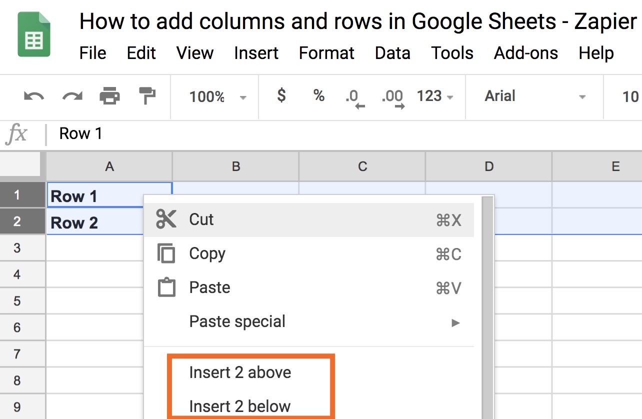
Method 2: Using the right-click menu

Select the column or columns you want to hide by clicking on the column header(s).
Right-click on the selected column header(s) to open the context menu.
Click on the “Hide column” option. The selected column(s) will be hidden.

Method 3: Using the keyboard shortcut

Select the column or columns you want to hide by clicking on the column header(s).
Press and hold the “Ctrl” key (Windows) or “Command” key (Mac).
Press the “0” (zero) key on your keyboard. The selected column(s) will be hidden.

Method 4: Using the “Hide” option in the “Format” menu

Select the column or columns you want to hide by clicking on the column header(s).
Click on the “Format” menu in the toolbar.
Hover over the “Hide” option, and a drop-down menu will appear.
Select the specific type of column(s) you want to hide, such as “Hide and skip” or “Hide and stop the movement of adjacent columns”.
The selected column(s) will now be hidden based on the chosen option.

Method 5: Hiding multiple columns at once

Select the first column you want to hide by clicking on its header.
Hold down the “Shift” key on your keyboard.
Select the last column you want to hide by clicking on its header.
All the columns between the first and last selected columns will be highlighted.
Follow any of the previously mentioned methods to hide the selected columns.

Method 6: Hiding columns permanently

Click on the “View” menu in the toolbar.
Hover over the “Hidden sheets” option, and a sub-menu will appear.
Click on “Hidden sheets” to open the “Hidden sheets” sidebar.
In the sidebar, you will see a list of hidden columns in your spreadsheet.
Select the column or columns you want to unhide by clicking on their checkboxes.
The selected column(s) will be unhidden and restored to their original positions.

By using these methods, you can easily hide columns in Google Sheets to declutter your view, focus on specific data, protect sensitive information, or present a clean and organized spreadsheet.

Method 1: Using the toolbar

One of the easiest ways to hide columns in Google Sheets is by using the toolbar. This method allows you to quickly hide individual columns or multiple columns at once. Here’s how:

Select the column or columns you want to hide by clicking on the column header(s). You can hold down the “Ctrl” key (Windows) or “Command” key (Mac) to select multiple columns.
Click on the “Format” menu in the toolbar at the top of the Google Sheets interface.
A dropdown menu will appear. Hover over the “Hide” option.
Another dropdown menu will appear with two options: “Hide row” and “Hide column”. Click on “Hide column”.

After completing these steps, the selected column(s) will be hidden from view in your spreadsheet. You will notice that the hidden column(s) no longer appear, and the adjacent columns will adjust accordingly to fill the space.

To unhide a hidden column using the toolbar, follow the same steps until you reach the “Hide column” option. However, instead of selecting it, you will see the option “Unhide column” in the dropdown menu. Click on “Unhide column” to reveal the previously hidden column(s).

The toolbar method is quick and straightforward, making it a convenient way to hide and unhide columns as needed. Whether you need to declutter your spreadsheet or focus on specific data, using the toolbar provides a user-friendly approach to organizing your columns in Google Sheets.

Method 2: Using the right-click menu

Another convenient method to hide columns in Google Sheets is by utilizing the right-click menu. This method allows you to quickly access the “Hide column” option with a simple right-click. Here’s how to do it:

Select the column or columns you want to hide by clicking on the column header(s). To select multiple columns, hold down the “Ctrl” key (Windows) or “Command” key (Mac) while clicking on the column headers.
After selecting the desired columns, right-click on any of the selected column headers. A context menu will appear.
In the right-click menu, locate and click on the “Hide column” option. Google Sheets will hide the selected column(s) from view.

Once hidden, the selected column(s) will no longer be visible in your spreadsheet. The adjacent columns will adjust to fill the space created by the hidden columns.

To unhide a hidden column using the right-click menu, follow the same steps as above, but instead of selecting “Hide column”, you will see the option “Unhide column” in the right-click menu. Click on “Unhide column” to reveal the previously hidden column(s).

The right-click menu method provides a quick and intuitive way to hide and unhide columns in Google Sheets. With just a few clicks, you can easily manage the visibility of columns in your spreadsheet to focus on relevant data or improve the overall layout.

Method 3: Using the keyboard shortcut

If you prefer using keyboard shortcuts to navigate and perform actions in Google Sheets, you’ll be pleased to know that there is a keyboard shortcut for hiding columns. This method allows you to hide columns with a simple combination of keys. Here’s how to do it:

Select the column or columns you want to hide by clicking on the column header(s). Hold down the “Ctrl” key (Windows) or “Command” key (Mac) to select multiple columns.
Once the desired columns are selected, press and hold the “Ctrl” key (Windows) or “Command” key (Mac) on your keyboard.
While holding the “Ctrl” or “Command” key, press the “0” (zero) key on your keyboard.

By pressing this keyboard shortcut, the selected column(s) will be hidden from view in your spreadsheet. The adjacent columns will automatically adjust to fill the space left by the hidden columns.

To unhide a hidden column using the keyboard shortcut, follow the same steps above to select the hidden column(s). Once selected, press the same keyboard shortcut combination: hold down the “Ctrl” (Windows) or “Command” (Mac) key, and press the “0” (zero) key. The hidden column(s) will be unhidden and reappear in your spreadsheet.

The keyboard shortcut method is a convenient way to hide and unhide columns in Google Sheets without needing to navigate through menus or use the mouse. It allows for quick and efficient management of column visibility, making it an ideal option for keyboard-centric users.

Method 4: Using the “Hide” option in the “Format” menu

The “Hide” option in the “Format” menu provides an alternative way to hide columns in Google Sheets. This method offers additional options for customizing the behavior of hidden columns. Here’s how to use this method:

Select the column or columns you want to hide by clicking on the column header(s).
Click on the “Format” menu in the toolbar at the top of the Google Sheets interface.
A dropdown menu will appear. Hover over the “Hide” option.
A sub-menu will open, presenting different options for hiding columns.
Select the specific option that suits your needs:
- “Hide column” will hide the selected column(s) while allowing adjacent columns to move and adjust automatically to fill the empty space created.
- “Hide and skip” will hide the column(s) and maintain a gap in the column sequence, ensuring that adjacent columns do not move or adjust.
- “Hide and stop the movement of adjacent columns” will hide the column(s) and freeze the adjacent columns in their current position, preventing them from moving or adjusting.

Once you’ve selected the desired hiding option, Google Sheets will hide the selected column(s) based on your chosen preference.

To unhide a column using this method, follow the same steps until you reach the “Hide” option in the “Format” menu. Instead of selecting “Hide column”, you will see the option “Unhide column” in the sub-menu. Click on “Unhide column” to reveal the previously hidden column(s).

The “Hide” option in the “Format” menu provides flexibility in hiding columns while preserving the formatting and behavior of the adjacent columns. By utilizing the different hiding options, you can choose the most suitable approach for your specific data organization and presentation needs.

Method 5: Hiding multiple columns at once

In Google Sheets, you have the option to hide multiple columns simultaneously, which can be a time-saving feature when dealing with large datasets or when you want to hide several columns at once. Here’s how you can hide multiple columns:

Select the first column you want to hide by clicking on its header.
While holding down the “Shift” key on your keyboard, select the last column you want to hide by clicking on its header.
All the columns between the first and last selected columns will be highlighted.
With the selected columns highlighted, use any of the aforementioned methods, such as the toolbar, right-click menu, or keyboard shortcut, to hide the selected columns.

Once you’ve hidden the selected columns, you’ll notice that they are no longer visible in your spreadsheet. The adjacent columns will automatically adjust to fill the space, providing a clean and organized view of your data.

To unhide multiple columns that were hidden together, follow the same steps to select the hidden columns. Then, use any of the methods mentioned earlier to unhide them. The previously hidden columns will be revealed and displayed in your spreadsheet again.

Hiding multiple columns at once allows for efficient management and organization of data within your spreadsheet. Whether you’re dealing with a complex analysis or simply need to declutter your view, this method enables you to hide multiple columns simultaneously, saving you time and effort.

Method 6: Hiding columns permanently

In certain cases, you may need to hide columns permanently, ensuring they remain hidden even when you close and reopen the spreadsheet. Google Sheets provides a solution to handle this scenario. Here’s how you can hide columns permanently:

Click on the “View” menu in the toolbar at the top of the Google Sheets interface.
From the dropdown menu, hover over the “Hidden sheets” option.
A sub-menu will appear, displaying a list of hidden columns in your spreadsheet.
Select the column or columns you want to unhide by clicking on their checkboxes. These columns will no longer be hidden and will be restored to their original positions in the spreadsheet.

By following this method, you can retrieve and unhide the hidden columns, making them visible in your spreadsheet once again.

It’s important to note that this method works for permanently hiding individual columns or groups of hidden columns. The “Hidden sheets” feature enables you to manage and restore hidden columns efficiently, ensuring you have control over the visibility of columns in your spreadsheet.

Keep in mind that the “Hidden sheets” feature is specific to hiding columns permanently and managing visibility, separate from other methods mentioned earlier that temporarily hide and unhide columns within a single session of Google Sheets.

By utilizing the “Hidden sheets” feature, you can confidently hide columns permanently without worrying about their visibility when reopening the spreadsheet. This method allows for enhanced data organization and customization, empowering you to maintain a clean and streamlined view in your Google Sheets.

Conclusion

Hiding columns in Google Sheets is a valuable feature that allows you to declutter your spreadsheet, focus on specific data, and customize the layout of your sheet. By utilizing the various methods outlined in this article, you have the flexibility to hide columns using the toolbar, right-click menu, keyboard shortcut, or the “Hide” option in the “Format” menu.

Whether you need to temporarily hide columns to eliminate distractions, protect sensitive information, or present a clean and organized view to others, Google Sheets offers versatile options. You can hide individual columns or multiple columns at once, and even choose how adjacent columns behave when the hidden columns are in effect.

Furthermore, for scenarios where you want to hide columns permanently, Google Sheets provides the “Hidden sheets” feature. This allows you to manage and restore hidden columns even when you close and reopen your spreadsheet.

By mastering these methods, you can optimize your data analysis, reporting, and collaboration workflows in Google Sheets. Customizing the visibility of columns empowers you to highlight relevant information, improve readability, and maintain data privacy when sharing your spreadsheets with others.

So, the next time your Google Sheets workspace feels cluttered or you need to present a focused view of your data, remember these methods for hiding columns. Experiment with them, find the approach that suits your needs best, and enjoy the benefits of a well-organized and visually appealing spreadsheet.