Introduction
Machine learning is an exciting field that has gained significant attention in recent years. With its ability to analyze and make predictions from data, machine learning has found applications in various domains, including finance, healthcare, and marketing. One of the fundamental concepts in machine learning is regression, which allows us to model and understand the relationships between variables.
Regression is a type of supervised learning technique that aims to predict a continuous target variable based on one or more input features. It helps us understand how the independent variables (input features) impact the dependent variable (target). By fitting a regression model to a dataset, we can estimate the relationship and make predictions for new data points.
There are various types of regression algorithms, each with its own strengths and assumptions. The choice of regression method depends on the nature of the data and the goal of the analysis. Some commonly used regression algorithms include linear regression, polynomial regression, lasso regression, ridge regression, and elastic net regression.
In this article, we will explore the different types of regression algorithms, understand their underlying principles, and discuss when to use each one. We will also delve into the evaluation metrics used to assess the performance of regression models and provide tips on how to improve their effectiveness.
Whether you are a data scientist, analyst, or business professional, understanding regression is crucial for making accurate predictions and informed decisions. By the end of this article, you will have a solid understanding of regression in machine learning and be ready to apply this powerful technique to your own data analysis tasks.
What is Regression?
Regression is a statistical modeling technique used in machine learning to predict or estimate the value of a continuous target variable based on one or more input features. It is a supervised learning algorithm, meaning that it requires labeled data with known outputs to learn the underlying relationship between the input features and the target variable.
The main goal of regression analysis is to understand the relationship between the independent variables (also known as predictors or features) and the dependent variable (the target). By fitting a regression model to the data, we aim to estimate the coefficients or weights that represent the strength and direction of the relationship.
Regression models can be used for various purposes, such as:
- Predicting the future value of a continuously varying metric, such as stock prices or housing prices.
- Analyzing the impact of independent variables on a dependent variable, such as understanding how advertising expenditure affects sales.
- Identifying key factors that influence a particular outcome, such as determining which features of a product contribute most to customer satisfaction.
Regression analysis assumes a linear relationship between the independent variables and the target variable. However, in practice, this relationship might not always be linear. Therefore, regression algorithms offer different variations to handle non-linear patterns and complex relationships.
Overall, regression is a powerful tool for understanding and predicting continuous variables. It provides valuable insights into how different variables impact the target variable, helping businesses make data-driven decisions and optimize their strategies.
Types of Regression
Regression models come in various forms, each with its own assumptions and characteristics. Understanding the different types of regression algorithms is essential for selecting the most appropriate model for your data. Here are some commonly used types of regression:
1. Linear Regression:
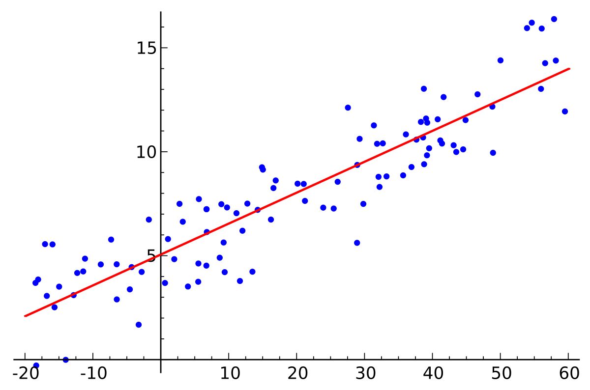
Linear regression is the most basic and widely used type of regression. It assumes a linear relationship between the independent variables and the target variable. The goal is to find the best-fit line that minimizes the distance between the observed data points and the line. Linear regression is suitable when the relationship between variables is expected to be linear.
2. Polynomial Regression:
Polynomial regression is an extension of linear regression that allows for non-linear relationships between variables. It involves transforming the original predictors into higher-degree polynomials, enabling the model to capture complex patterns. Polynomial regression is useful when the relationship between variables is curved or has peaks and valleys.
3. Lasso Regression:
Lasso regression (Least Absolute Shrinkage and Selection Operator) is a regularization technique that adds a penalty term to the linear regression objective function. This penalty encourages the model to select fewer variables and use only the most important features, effectively reducing model complexity and preventing overfitting. Lasso regression is particularly useful when dealing with high-dimensional datasets.
4. Ridge Regression:
Ridge regression is another regularization technique similar to lasso regression. It also adds a penalty term to the linear regression objective function but uses the squared magnitude of the coefficients instead. This penalty term shrinks the coefficient values, reducing the impact of less important features. Ridge regression helps overcome issues like multicollinearity and improves model stability.
5. Elastic Net Regression:
Elastic net regression combines the strengths of lasso and ridge regression. It applies both L1 and L2 penalties to the objective function, allowing for variable selection and coefficient shrinkage. Elastic net regression is effective in situations where there is multicollinearity and many potentially relevant features.
These are just a few examples of regression algorithms, and there are other specialized variations depending on the specific requirements and characteristics of the data. Choosing the right type of regression algorithm depends on the nature of the problem and the characteristics of the dataset. It is important to experiment with different models and evaluate their performance to select the most suitable one for your task.
Linear Regression
Linear regression is a widely used statistical technique for modeling the relationship between independent variables and a continuous target variable. It assumes a linear relationship between the input features and the target variable, which can be represented by a straight line in a two-dimensional space or a hyperplane in higher dimensions.
The goal of linear regression is to find the best-fit line that minimizes the sum of squared differences between the observed data points and the predicted values. The line is determined by estimating the coefficients or weights that represent the slope and intercept of the line.
The equation for a simple linear regression model with one independent variable can be expressed as:
y = b0 + b1 * x
Where:
– y is the dependent variable or the target variable.
– x is the independent variable.
– b0 is the y-intercept or the constant term.
– b1 is the slope coefficient of the independent variable.
The coefficient b1 represents the change in the target variable for a one-unit increase in the independent variable, assuming all other variables remain constant. The coefficient b0 represents the value of the target variable when the independent variable is zero.
Linear regression can be extended to multiple independent variables, resulting in multiple linear regression. The equation for multiple linear regression can be expressed as:
y = b0 + b1 * x1 + b2 * x2 + … + bn * xn
Where x1, x2, …, xn represent the values of the independent variables, and b1, b2, …, bn represent the corresponding slope coefficients.
Linear regression is commonly used for prediction and inference tasks in various domains. It provides valuable insights into the relationship between variables and can be used for forecasting, trend analysis, and understanding the impact of different factors on the target variable.
It’s important to note that linear regression assumes a linear relationship between the variables. If the relationship is more complex or non-linear, other regression techniques like polynomial regression or non-linear regression may be more appropriate.
Polynomial Regression
Polynomial Regression is an extension of linear regression that allows for modeling non-linear relationships between independent variables and a continuous target variable. It is a flexible regression technique that can capture more complex patterns in the data by introducing polynomial terms.
In polynomial regression, we transform the original predictors (independent variables) into higher-degree polynomials. By including these polynomial terms in the regression equation, the model can better fit the data and account for the curvature or non-linear relationship between the variables.
The equation for polynomial regression can be expressed as:
y = b0 + b1 * x + b2 * x^2 + … + bn * x^n
Where x represents the independent variable, y is the target variable, and b0, b1, …, bn are the coefficients or weights associated with each corresponding polynomial term.
By including higher-degree polynomial terms (such as quadratic or cubic terms), the model can capture more intricate relationships and better represent the non-linear behavior of the data.
Polynomial regression is useful when the relationship between the variables is not linear and shows curves, peaks, valleys, or other non-linear patterns. It is commonly used in areas such as physics, engineering, economics, and social sciences to model phenomena that exhibit non-linear behavior.
However, it is important to exercise caution when using polynomial regression, as including high-degree polynomial terms can lead to overfitting if not properly regularized. Overfitting occurs when the model becomes too complex and captures noise or random variations in the data instead of the actual underlying relationship. Regularization techniques such as ridge or lasso regression can be applied to mitigate the risk of overfitting in polynomial regression models.
Overall, polynomial regression provides a flexible and powerful approach for capturing non-linear relationships between variables. It allows for more accurate modeling of complex phenomena and can yield better predictions and insights compared to linear regression when dealing with non-linear data.
Lasso Regression
Lasso regression, short for Least Absolute Shrinkage and Selection Operator, is a regularization technique used in linear regression. It is especially useful when dealing with datasets that have a large number of features or predictors, as it helps with variable selection and mitigates the risk of overfitting.
In lasso regression, a penalty term is added to the linear regression objective function. This penalty term is the sum of the absolute values of the coefficients multiplied by a tuning parameter, which controls the amount of regularization applied. The objective is to minimize the sum of squared differences between the observed data points and the predicted values, while also keeping the magnitudes of the coefficients as small as possible.
One of the key advantages of lasso regression is that it can drive some of the coefficient values to exactly zero. This feature makes lasso regression useful for feature selection by identifying and discarding irrelevant or less important features. The resulting sparse regression model can provide a more interpretable and simplified representation of the data, focusing only on the most influential features.
Lasso regression is particularly effective in situations where there are a large number of features but only a few of them are expected to have a significant impact on the target variable. It can be used for both numerical and categorical predictors, making it a versatile technique for a wide range of applications.
It is important to carefully select the value of the tuning parameter, also known as the regularization parameter or lambda. A small lambda value results in minimal regularization, and the lasso regression model will behave similarly to a standard linear regression. On the other hand, a large lambda value increases the amount of regularization, leading to more coefficients being shrunk towards zero.
Lasso regression has applications in various domains, including finance, bioinformatics, and social sciences. It is a valuable tool for variable selection, identifying the most important predictors, and reducing model complexity in high-dimensional datasets.
Overall, lasso regression provides a useful approach for regularizing linear regression models and facilitating feature selection. By penalizing the absolute values of the coefficients, it allows for a simpler and more interpretable model while still maintaining good predictive performance.
Ridge Regression
Ridge regression is a regularization technique used in linear regression to tackle the issue of multicollinearity and improve the stability of the model. It is particularly useful when dealing with datasets that have highly correlated features or predictors.
Similar to lasso regression, ridge regression adds a penalty term to the linear regression objective function. However, instead of using the sum of absolute values of the coefficients, ridge regression utilizes the sum of squared values, multiplied by a tuning parameter known as the regularization parameter or lambda. The objective is to minimize the sum of squared differences between the observed data points and the predicted values, while also keeping the magnitudes of the coefficients as small as possible.
Ridge regression has a notable effect on the coefficient values – it shrinks them towards zero, but without driving any of them to exactly zero. This means that ridge regression retains all the predictors and does not perform variable selection like lasso regression does. Instead, it reduces the impact of less important features by shrinking their coefficient values.
Ridge regression helps address the issue of multicollinearity, which occurs when two or more predictors in a dataset are highly correlated. In such cases, standard linear regression models can produce unstable and unreliable coefficient estimates. By introducing the ridge penalty, ridge regression reduces the impact of multicollinearity and provides more reliable coefficient estimates.
Choosing the appropriate value for the regularization parameter, lambda, is crucial in ridge regression. A smaller lambda value results in less regularization, and the ridge regression model becomes similar to a standard linear regression. In contrast, a larger lambda value increases the regularization effect, shrinking the coefficients more towards zero.
Ridge regression has applications in various fields, such as finance, genetics, and image analysis. It is particularly useful when dealing with datasets that have many predictors and high collinearity among them.
Overall, ridge regression provides a valuable method for improving the stability and reliability of linear regression models in the presence of multicollinearity. By shrinking the coefficient values and reducing the impact of less important features, ridge regression offers a more robust approach to regression analysis.
Elastic Net Regression
Elastic Net regression is a regularization technique that combines the strengths of both lasso regression and ridge regression. It is particularly useful when dealing with high-dimensional datasets that exhibit multicollinearity and require feature selection.
Similar to lasso and ridge regression, elastic net regression adds a penalty term to the linear regression objective function. The penalty term combines both the L1 norm (absolute values of coefficients) and the L2 norm (squared values of coefficients), which are multiplied by a tuning parameter called alpha. This dual regularization allows elastic net regression to perform both variable selection and coefficient shrinkage.
The equation for elastic net regression can be expressed as:
y = b0 + b1 * x1 + b2 * x2 + … + bn * xn + lambda * (alpha * (sum(|b1|) + sum(b2^2)) + (1 – alpha) * (sum(|b1|) + sum(b2^2)))
Where x1, x2, …, xn represent the independent variables, y is the target variable, b0, b1, …, bn are the coefficients or weights, and lambda controls the overall amount of regularization.
Elastic net regression strikes a balance between the feature selection capability of lasso regression and the stability of ridge regression. The parameter alpha determines the proportion of L1 and L2 penalties in the regularization term. By adjusting the value of alpha, one can control the degree to which elastic net regression emphasizes feature selection versus coefficient shrinkage.
Elastic net regression is advantageous when dealing with datasets that have a large number of features and when there is multicollinearity among the predictors. It can effectively handle situations where there are more variables than observations and can provide robust and interpretable models.
Choosing the appropriate values for the regularization parameter, lambda, and the proportion parameter, alpha, is crucial in elastic net regression. Cross-validation techniques can be employed to find the optimal values that yield the best performance on the given dataset.
Overall, elastic net regression offers a powerful regularization technique that combines the advantages of both lasso and ridge regression. It provides a comprehensive approach to handle high-dimensional datasets, multicollinearity, and feature selection, making it a valuable tool for regression analysis in various domains.
When to Use Regression?
Regression analysis is a versatile and widely used statistical technique that can be employed in various scenarios. Here are some situations where regression analysis is applicable and useful:
1. Predictive Modeling:
Regression is commonly used for predictive modeling, where the goal is to estimate or forecast a continuous target variable based on the values of independent variables. By analyzing the relationship between the predictors and the target, regression models can make accurate predictions, such as predicting future sales, stock prices, or customer churn rates.
2. Relationship Assessment:
Regression analysis helps assess the strength and nature of the relationships between variables. It allows us to quantify the impact of independent variables on the dependent variable and understand the direction and magnitude of these relationships. This is particularly valuable in fields like economics, social sciences, and marketing, where understanding causal relationships is crucial.
3. Trend Analysis:
Regression can be used to identify and analyze trends in data. By fitting a regression line to the observed data points, we can determine whether there is a consistent upward or downward trend over time. This is useful for identifying patterns, making forecasts, and formulating strategies based on historical data.
4. Estimating Impact:
Regression analysis is useful for estimating the impact of independent variables on a dependent variable. For example, in marketing, regression can be applied to understand how changes in advertising expenditure impact sales. By quantifying the relationship, businesses can make informed decisions about resource allocation and optimization.
5. Outlier Detection:
Regression analysis can help identify outliers, which are data points that deviate significantly from the expected patterns. Outliers can distort the regression line and impact the accuracy of predictions. By detecting and handling outliers, regression models can be improved and made more robust.
Overall, regression analysis is applicable in a wide range of fields and can be useful for various purposes, such as prediction, relationship assessment, trend analysis, and outlier detection. It allows for data-driven decision making, helps understand complex processes, and provides valuable insights into the relationships between variables.
How Does Regression Work?
Regression is a statistical modeling technique that aims to understand and predict the relationship between independent variables (predictors) and a dependent variable (target). The goal is to estimate the coefficients or weights that describe the strength and direction of the relationship, allowing us to make predictions for new data points.
The regression process involves several key steps:
1. Data Collection:
The first step in regression analysis is gathering the necessary data. This includes collecting observations of the dependent variable and measuring the corresponding values of the independent variables. The data should be representative of the population or phenomenon being studied.
2. Data Preprocessing:
Before fitting a regression model, it is essential to preprocess the data. This involves handling missing values, dealing with outliers, scaling or standardizing variables, and transforming variables if necessary. Data preprocessing ensures that the data is suitable for regression analysis and helps improve the model’s performance.
3. Model Selection:
Choosing the appropriate regression model is crucial. There are different types of regression algorithms available, such as linear regression, polynomial regression, lasso regression, ridge regression, and elastic net regression. The selection depends on the nature of the data, the relationship being investigated, and the assumptions of the model.
4. Model Training:
Once a regression model is selected, the next step is to train the model using the collected data. This involves estimating the coefficients or weights that define the relationship between the independent variables and the dependent variable. The training process uses optimization techniques to find the best-fit values that minimize the difference between the predicted values and the actual observed values.
5. Model Evaluation:
To assess the performance of the regression model and its ability to make accurate predictions, evaluation metrics are used. Commonly used evaluation metrics for regression include mean squared error (MSE), root mean squared error (RMSE), mean absolute error (MAE), and R-squared. These metrics help gauge how well the model fits the data and how well it generalizes to unseen data.
6. Model Deployment and Prediction:
Once the regression model is trained and evaluated, it can be deployed for making predictions on new data. The model takes the values of the independent variables as input and produces a predicted value for the dependent variable. These predictions can be used for inference, decision making, or forecasting future outcomes.
By following these steps, regression analysis enables us to gain insights into relationships between variables, make predictions, and inform decision making in various fields and industries.
Evaluation Metrics for Regression
Evaluation metrics for regression models provide a means to assess the performance and accuracy of the predictions made by the model. These metrics help quantify the difference between the predicted values and the true observed values, providing insight into how well the model fits the data. Here are some commonly used evaluation metrics for regression:
1. Mean Squared Error (MSE):
MSE calculates the average squared difference between the predicted and actual values. It provides a measure of the overall model performance, with lower values indicating better accuracy. However, MSE is sensitive to outliers as it squares the differences, amplifying their impact.
2. Root Mean Squared Error (RMSE):
RMSE is the square root of MSE and provides a measure of the average difference between the predicted and actual values. It is particularly useful for interpretability, as it is on the same scale as the target variable. Like MSE, a lower RMSE indicates better performance.
3. Mean Absolute Error (MAE):
MAE calculates the average absolute difference between the predicted and actual values. It is less sensitive to outliers compared to MSE as it doesn’t square the differences. MAE provides a robust measure of model performance and is easy to interpret as it is on the same scale as the target variable.
4. R-squared (R^2):
R-squared represents the proportion of the variance in the dependent variable that is explained by the independent variables. It ranges from 0 to 1, with a value of 1 indicating a perfect fit. R-squared provides an indication of how well the model captures the variability in the data, with higher values representing better fit.
5. Adjusted R-squared:
Adjusted R-squared adjusts for the number of predictors in the model. It penalizes the inclusion of irrelevant predictors and helps prevent overfitting. Adjusted R-squared provides a more accurate measure of how well the model generalizes to new data, taking into account the complexity of the model.
6. Mean Percentage Error (MPE):
MPE measures the average percentage difference between the predicted and actual values. It provides insight into the direction and magnitude of the prediction errors. A positive MPE indicates an overestimation, while a negative MPE indicates an underestimation of the target variable.
Evaluation metrics serve as quantitative measures to assess different aspects of a regression model’s performance. The selection of an appropriate metric depends on the specific goals, requirements, and characteristics of the problem at hand. These metrics provide valuable insights into how well the model is performing and help guide improvements and refinements to the model, if necessary.
Tips for Improving Regression Models
Improving the performance and effectiveness of regression models can lead to more accurate predictions and better insights. Here are some tips to consider when working with regression models:
1. Feature Engineering:
Feature engineering involves transforming and creating new features from the existing ones to better represent the underlying relationship between the predictors and the target variable. This may include polynomial transformations, interaction terms, or creating meaningful categorical variables. Thoughtful feature engineering can enhance model performance by capturing complex patterns and improving the model’s ability to generalize.
2. Dealing with Missing Data:
Missing data can adversely impact the performance of regression models. It is important to assess the extent of missingness and handle missing values appropriately. This can be done through techniques such as imputation, where missing values are estimated using statistical methods, or using algorithms that can handle missing data directly.
3. Handling Outliers:
Outliers can significantly affect regression models, leading to biased parameter estimates and decreased predictive accuracy. It is crucial to identify and handle outliers effectively. This can involve techniques such as winsorization, where extreme values are replaced with less extreme values, or removing outliers based on statistical criteria. Consider the impact of outliers on the relationship between variables and choose an appropriate approach accordingly.
4. Regularization Techniques:
Implementing regularization techniques like lasso regression, ridge regression, or elastic net regression can help improve the stability and generalization of the regression model. Regularization helps prevent overfitting by shrinking or selecting coefficients, reducing the model’s complexity and improving its ability to perform well on unseen data.
5. Cross-Validation:
Utilize cross-validation techniques to evaluate the performance of the regression model. Cross-validation splits the data into training and validation sets, allowing for an unbiased assessment of the model’s predictive ability. K-fold cross-validation, leave-one-out cross-validation, or bootstrapping techniques can provide robust estimates of the model’s performance and assist in selecting the best-performing model.
6. Feature Selection:
Perform feature selection to identify the most important predictors for your regression model. Approaches such as backward elimination, forward selection, or stepwise regression can help identify the subset of variables that contribute the most to the model’s predictive power. Feature selection reduces overfitting, enhances model interpretability, and improves computational efficiency.
Remember that improving regression models is an iterative process that requires experimentation, evaluation, and refinement. Continuously assess the model’s performance, consider alternative approaches, and iteratively implement improvements to achieve the best results.
Conclusion
Regression analysis is a powerful and widely used statistical technique that allows us to model and understand the relationships between variables. Whether we need to predict future outcomes, estimate the impact of independent variables, or assess the strength of relationships, regression provides valuable insights and helps make informed decisions.
Throughout this article, we have explored the basics of regression, including its definition and types. We discussed linear regression, polynomial regression, lasso regression, ridge regression, and elastic net regression, each with its own characteristics and applications.
We also covered important aspects such as when regression analysis is appropriate, how regression works, and the evaluation metrics used to assess model performance. Understanding these elements is crucial for effectively applying regression techniques to real-world problems.
Additionally, we provided tips for improving regression models, such as feature engineering, dealing with missing data and outliers, employing regularization techniques, utilizing cross-validation, and performing feature selection. These practices can enhance the performance, stability, and interpretability of regression models, leading to more accurate predictions and better insights.
In conclusion and as we wrap up, regression analysis serves as a fundamental tool in the field of machine learning and data analysis. Its ability to uncover relationships, make predictions, and guide decision-making makes it a valuable technique in numerous domains. By leveraging the concepts and tips provided in this article, you can confidently apply regression analysis to your own data analysis tasks and unlock its power in solving complex problems.