Introduction
Welcome to the fascinating world of machine learning! As the field continues to evolve, it’s crucial to understand the various tools and concepts that help us analyze and evaluate our models’ performance. One such tool is the confusion matrix.
In machine learning, predicting outcomes accurately is a primary goal. However, it’s not always easy to determine how well our model is performing just by looking at the overall accuracy. This is where the confusion matrix comes into play. It provides us with a more detailed understanding of our model’s predictions – allowing us to effectively evaluate its strengths and weaknesses.
The confusion matrix, also known as an error matrix, is a performance measurement tool used in supervised learning tasks. It allows us to visualize the performance of a classification model by classifying and categorizing the predicted and actual values. By showing the true positive, true negative, false positive, and false negative values, the confusion matrix gives us a clear picture of how well our model is performing.
This concept is essential because different classification tasks have different priorities. For instance, in a medical diagnosis scenario, correctly identifying a patient with a disease as positive (true positive) is crucial to providing them with appropriate treatment. On the other hand, wrongly classifying a healthy person as positive (false positive) can lead to unnecessary medical procedures or anxiety for the patient.
Understanding the confusion matrix allows data scientists and machine learning practitioners to go beyond simple accuracy measurements and gain deeper insights into the performance of their models. Through the confusion matrix, we can calculate various evaluation metrics such as precision, recall, F1-score, and specificity, enabling us to assess the model’s precision, sensitivity, overall performance, and ability to correctly classify instances.
In the following sections, we will explore how the confusion matrix works, its anatomy, and the evaluation metrics derived from it. Additionally, we will provide an example to illustrate the practical application of the confusion matrix in evaluating a classification model’s performance. So, let’s dive in!
What is a Confusion Matrix?
In the field of machine learning, a confusion matrix is a graphical representation of the performance of a classification model. It helps us evaluate the accuracy and effectiveness of our model’s predictions by comparing the predicted and actual values of a given dataset. The confusion matrix provides valuable insights into the types of errors our model is making and allows us to assess its strengths and weaknesses.
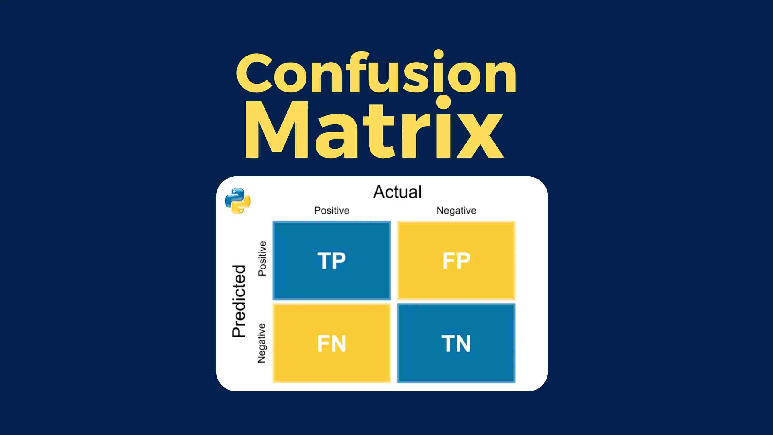
At its core, a confusion matrix is a 2×2 table that organizes the model’s predictions into four different categories:
- True Positives (TP): These are the instances where the model correctly predicted a positive outcome.
- True Negatives (TN): These are the instances where the model correctly predicted a negative outcome.
- False Positives (FP): These are the instances where the model incorrectly predicted a positive outcome when the actual value was negative.
- False Negatives (FN): These are the instances where the model incorrectly predicted a negative outcome when the actual value was positive.
The confusion matrix provides us with a detailed breakdown of the model’s performance by quantifying the number of instances that fall into each category. By examining these numbers, we can calculate several key evaluation metrics that offer a more comprehensive assessment of the model’s accuracy and effectiveness.
One important aspect of the confusion matrix is that it is typically used in classification tasks, where the outcome is divided into discrete classes or categories. However, it can also be adapted for multiclass classification problems by expanding it to include more categories.
Overall, the confusion matrix plays a vital role in understanding and evaluating the performance of classification models. It goes beyond simple accuracy measurements and provides a deeper analysis of the types of errors being made. By utilizing the confusion matrix, we can make more informed decisions about our model’s performance and take appropriate steps to improve its accuracy and effectiveness.
Why is the Confusion Matrix Important in Machine Learning?
The confusion matrix is a critical tool in machine learning as it provides valuable insights into the performance of classification models. By examining the confusion matrix, we can gain a deeper understanding of how well our model is performing, beyond a simple accuracy score.
One of the main reasons why the confusion matrix is important is that it allows us to identify different types of errors made by our model. These errors can have varying levels of impact and consequences depending on the specific application. For example, in a cancer diagnosis scenario, a false negative (predicting a healthy patient as having cancer) can have severe implications, leading to potentially delayed treatment. However, a false positive (predicting a healthy patient as having cancer) can also cause unnecessary stress and medical procedures. By analyzing the confusion matrix, we can identify these errors and take appropriate actions to minimize them.
Furthermore, the confusion matrix provides us with key evaluation metrics that can help us assess the performance of our model. Some of the commonly derived metrics from the confusion matrix include:
- Accuracy: Measures the overall correctness of the model’s predictions.
- Precision: Indicates the proportion of true positive predictions among all positive predictions, providing insights into the model’s ability to avoid false positives.
- Recall: Measures the proportion of actual positive instances that the model correctly identifies as positive, reflecting the model’s sensitivity in detecting positive cases.
- F1-score: Combines precision and recall to provide a balanced evaluation of the model’s performance.
- Specificity: Measures the proportion of actual negative instances that the model correctly identifies as negative, highlighting the model’s ability to avoid false negatives.
These metrics derived from the confusion matrix give us a more comprehensive understanding of our model’s strengths and weaknesses. By assessing these metrics, we can gauge the model’s reliability, sensitivity, precision, and overall capability to classify instances accurately.
Moreover, the confusion matrix is essential for model optimization and improvement. By studying the patterns within the matrix, we can identify specific areas where the model is struggling and take proactive steps to address those weaknesses. For example, if the model consistently has high false positive rates, we can adjust the threshold or fine-tune the model to minimize these errors.
Overall, the confusion matrix is a crucial tool in machine learning as it provides a comprehensive evaluation of classification model performance. It helps us understand the types of errors our model is making, calculate important evaluation metrics, and identify areas for improvement. By leveraging the insights from the confusion matrix, we can make informed decisions to enhance the accuracy and effectiveness of our machine learning models.
How Does a Confusion Matrix Work?
The confusion matrix is a powerful tool in machine learning that provides a detailed breakdown of a classification model’s performance. It works by comparing the predicted and actual values of a dataset and organizing them into a matrix of four categories: true positives (TP), true negatives (TN), false positives (FP), and false negatives (FN).
Let’s understand how the confusion matrix works through the following steps:
- Data Split: The dataset is split into training and testing sets.
- Model Training: The classification model is trained using the training set to learn patterns and make predictions.
- Prediction: The trained model is used to predict the classes of the instances in the testing set.
- Comparison: The predicted values are compared to the actual values of the testing set.
- Matrix Construction: Using the comparison results, a confusion matrix is constructed to summarize the model’s performance.
The confusion matrix is typically represented as a 2×2 table with rows representing the actual values and columns representing the predicted values. The four categories of the confusion matrix are defined as follows:
- True Positives (TP): These are instances where the model correctly predicted a positive outcome.
- True Negatives (TN): These are instances where the model correctly predicted a negative outcome.
- False Positives (FP): These are instances where the model incorrectly predicted a positive outcome when the actual value was negative.
- False Negatives (FN): These are instances where the model incorrectly predicted a negative outcome when the actual value was positive.
By organizing the predictions into these categories, the confusion matrix provides us with a clear breakdown of the model’s performance. Each cell in the matrix represents the count or percentage of instances falling into a particular category.
From this matrix, we can calculate various evaluation metrics such as accuracy, precision, recall, F1-score, and specificity. These metrics allow us to assess the model’s overall performance, sensitivity, specificity, and ability to accurately classify instances.
Through the confusion matrix, we gain deeper insights into how well our model is performing. It allows us to identify the types of errors it is making and make informed decisions to improve its accuracy and effectiveness. By utilizing the power of the confusion matrix, we can optimize our classification models and make more accurate predictions.
Anatomy of a Confusion Matrix
To understand and interpret a confusion matrix correctly, it’s essential to familiarize ourselves with its components. The anatomy of a confusion matrix consists of four main elements: true positives (TP), true negatives (TN), false positives (FP), and false negatives (FN).
True Positives (TP): This refers to the number of instances that are correctly classified as positive by the model. In other words, TP represents the cases where the model predicted a positive outcome, and the actual value was indeed positive. For example, in a medical diagnosis scenario, TP would be the number of correctly identified patients with a specific disease.
True Negatives (TN): TN represents the number of instances that are correctly classified as negative by the model. These are cases where the model predicted a negative outcome, and the actual value was negative. For instance, in an email spam detection model, TN would be the number of correctly identified non-spam emails.
False Positives (FP): FP refers to the number of instances that are incorrectly classified as positive by the model. These are cases where the model predicted a positive outcome, but the actual value was negative. In other words, the model has a false alarm and mistakenly classified a negative instance as positive. In the email spam detection example, FP would represent the number of non-spam emails classified as spam.
False Negatives (FN): FN indicates the number of instances that are incorrectly classified as negative by the model. These are cases where the model predicted a negative outcome, but the actual value was positive. FN represents instances that the model missed or failed to identify correctly. In the medical diagnosis scenario, FN would be the number of patients with the disease that were not correctly identified.
The correct interpretation and understanding of these elements in the confusion matrix are crucial for evaluating the model’s performance. By analyzing the values in each cell of the confusion matrix, we can derive meaningful evaluation metrics and gain insight into the model’s accuracy, precision, recall, and overall effectiveness.
Furthermore, it’s worth noting that the total number of instances in a dataset can be obtained by summing all the values in the confusion matrix. This information is valuable for calculating evaluation metrics such as accuracy, which measures the proportion of correctly classified instances out of the total.
With a clear understanding of the anatomy of a confusion matrix, we can leverage its insights to assess the performance of our classification models accurately. By analyzing the true positives, true negatives, false positives, and false negatives, we can evaluate the model’s strengths, weaknesses, and areas that require improvement.
Evaluation Metrics Derived from the Confusion Matrix
The confusion matrix provides us with a wealth of information about the performance of a classification model. By analyzing the values within the matrix, we can calculate several evaluation metrics that offer a more comprehensive assessment of the model’s effectiveness. These metrics provide insights into various aspects of the model’s performance, including accuracy, precision, recall, F1-score, and specificity.
Accuracy: Accuracy is a commonly used evaluation metric derived from the confusion matrix. It measures the overall correctness of the model’s predictions by calculating the ratio between the sum of true positives (TP) and true negatives (TN) to the total number of instances. Accuracy helps determine the proportion of correct predictions made by the model, providing a general measure of its performance.
Precision: Precision, also known as the positive predictive value, focuses on the proportion of true positives out of all instances predicted as positive (TP + FP). Precision provides insights into the model’s ability to avoid false positives. A high precision indicates that the model rarely misclassifies negative instances as positive, making it valuable in scenarios where false positives are costly or undesirable.
Recall: Recall, also known as sensitivity or true positive rate, measures the proportion of actual positive instances that the model correctly identifies as positive (TP). It evaluates the model’s ability to detect positive cases correctly. A high recall indicates that the model rarely misses positive instances, making it valuable in scenarios where it’s crucial to minimize false negatives, such as disease diagnosis or fraud detection.
F1-score: The F1-score is a weighted metric that combines precision and recall into a single value, providing a balanced evaluation of the model’s performance. It is calculated as the harmonic mean of precision and recall, and it ranges from 0 to 1. The F1-score helps gauge the overall effectiveness of the model, considering both its ability to avoid false positives and false negatives. A higher F1-score implies a better balance between precision and recall.
Specificity: Specificity, also known as the true negative rate, measures the proportion of actual negative instances that the model correctly identifies as negative (TN). It evaluates the model’s ability to avoid false negatives. A high specificity indicates that the model rarely misclassifies positive instances as negative, making it valuable in scenarios where false negatives are costly or undesirable.
These evaluation metrics derived from the confusion matrix provide valuable insights into different aspects of the model’s performance. By calculating and analyzing these metrics, we can assess the model’s accuracy, precision, recall, and ability to correctly classify instances. These metrics help us make informed decisions about model optimization, development of threshold criteria, or comparing the performance of different models and algorithms.
Accuracy
Accuracy is a widely used evaluation metric that measures the overall correctness of predictions made by a classification model. It quantifies the ratio of correctly classified instances (true positives and true negatives) to the total number of instances in the dataset.
The accuracy metric derived from the confusion matrix is calculated using the following formula:
Accuracy = (TP + TN) / (TP + TN + FP + FN)
Accuracy provides a general measure of a model’s performance, reflecting how often it correctly predicts the class labels. A high accuracy score indicates that the model is making correct predictions the majority of the time, while a low accuracy score indicates that the model’s predictions are less reliable.
While accuracy is a straightforward and intuitive metric, it may not always provide a complete picture of a model’s performance. Accuracy alone can be misleading, especially in cases where the dataset is imbalanced or the misclassification of certain classes carries more significant consequences.
In scenarios where class imbalance exists, where the number of instances in one class substantially outweighs the others, accuracy alone can be misleading. A model that predicts the majority class for all instances may achieve high accuracy, but it might not be adequately capturing the nuances of the minority class.
Additionally, if certain misclassifications are more detrimental than others, accuracy may not provide a comprehensive assessment. For example, in a medical diagnosis scenario, incorrectly classifying a patient with a severe condition as healthy (false negative) could have severe consequences. In this case, precision, recall, or other metrics may be more appropriate to evaluate the model’s performance.
Therefore, while accuracy is a valuable metric to give a broad overview of a model’s performance, it is important to consider other metrics derived from the confusion matrix, such as precision, recall, and F1-score, to gain more comprehensive insights. By assessing a combination of evaluation metrics, we can better understand the strengths and weaknesses of a classification model and make more informed decisions regarding its optimization and performance improvement.
Precision
Precision is an important evaluation metric derived from the confusion matrix that measures the proportion of true positive predictions out of all instances predicted as positive. It focuses on the model’s ability to avoid false positives, making it particularly relevant in situations where incorrectly classifying negative instances as positive has significant consequences.
Precision is calculated using the following formula:
Precision = TP / (TP + FP)
The precision metric provides insights into how well the model performs in classifying positive instances accurately. A high precision value indicates that the model has a low rate of false positives, meaning it rarely misclassifies negative instances as positive. On the other hand, a low precision value suggests that the model has a higher tendency to generate false positive predictions.
In certain applications, such as medical diagnoses or spam email detection, precision is of utmost importance. For example, in a medical context, a high precision value means that the model is correctly identifying patients with a specific disease, reducing the number of false positives that could lead to unnecessary treatments or interventions.
However, it’s crucial to note that optimizing for precision may come at the cost of higher false negative rates. If the model becomes overly cautious in classifying positive instances, it may miss some true positive cases. Therefore, the trade-off between precision and recall (also known as the precision-recall trade-off) should be considered based on the specific requirements and consequences of misclassifications in the given application.
To evaluate the model’s performance comprehensively, precision should be considered along with other metrics such as recall, accuracy, and F1-score. Combined, these metrics provide a more holistic understanding of the model’s classification performance, allowing us to make informed decisions regarding optimization, fine-tuning, and comparing different models or algorithms.
Recall
Recall, also known as sensitivity or true positive rate, is an important evaluation metric derived from the confusion matrix. It measures the proportion of actual positive instances that the model correctly identifies as positive. Recall is especially valuable in scenarios where correctly identifying positive cases is crucial and false negatives should be minimized.
Recall is calculated using the following formula:
Recall = TP / (TP + FN)
The recall metric provides insights into the model’s ability to capture positive instances accurately. A high recall value indicates that the model rarely misses positive cases, correctly identifying most of the instances that belong to the positive class. Conversely, a low recall value suggests that the model has a higher tendency to generate false negatives by incorrectly classifying positive instances as negative.
In various real-world applications, such as disease diagnostics or fraud detection, recall plays a critical role. In medical contexts, for example, a high recall value implies that the model is effectively identifying patients with a specific disease, minimizing the chances of false negatives that could lead to delayed treatment and adverse consequences.
It’s important to understand that optimizing for recall may result in higher false positive rates. By being more liberal in classifying instances as positive, the model may generate more false positives. Therefore, the trade-off between recall and precision should be carefully considered based on the specific requirements and consequences of misclassifications in a given application.
To evaluate the model’s performance holistically, recall should be considered together with other metrics, such as precision, accuracy, and F1-score. These metrics provide a comprehensive understanding of the model’s classification performance, allowing for informed decisions regarding optimization, fine-tuning, and comparisons between different models or algorithms.
F1-Score
The F1-score is a widely used evaluation metric derived from the confusion matrix that provides a balanced assessment of a classification model’s performance. It combines precision and recall into a single value, offering a robust evaluation of both the model’s ability to avoid false positives and false negatives.
The F1-score is calculated using the following formula:
F1-Score = 2 * (Precision * Recall) / (Precision + Recall)
The F1-score takes into account both precision and recall, providing a measure that strikes a balance between the two. The harmonic mean (instead of a simple arithmetic mean) is used to ensure that the F1-score gives equal emphasis to both precision and recall.
A high F1-score indicates that the model has performed well in terms of both avoiding false positives and minimizing false negatives. It reflects a good balance between precision and recall, indicating that the model is accurate in classifying positive instances while minimizing the misclassification of negative instances.
The F1-score is particularly useful when the distribution of classes is imbalanced, or when both precision and recall are equally important. For example, in an information retrieval system, precision is crucial to ensure the relevance of the retrieved documents, while recall is essential to cover as many relevant documents as possible.
By considering the F1-score alongside other evaluation metrics derived from the confusion matrix, such as accuracy, precision, and recall, we can gain a comprehensive understanding of a classification model’s performance. This allows us to make informed decisions regarding model optimization, threshold selection, or comparisons between different models or algorithms.
However, it’s important to note that the F1-score may not always be the ideal metric in every scenario. Depending on the specific application and the trade-off between precision and recall, other metrics may be more suitable for assessing a model’s performance. Therefore, it’s crucial to consider the context and requirements of the problem at hand when selecting evaluation metrics.
Specificity
Specificity is an essential evaluation metric derived from the confusion matrix that measures the proportion of actual negative instances that the model correctly identifies as negative. It complements recall by focusing on the model’s ability to avoid false negatives and is particularly relevant in scenarios where misclassifying negative instances as positive is undesirable.
Specificity is calculated using the following formula:
Specificity = TN / (TN + FP)
The specificity metric provides insights into how well the model performs in classifying negative instances correctly. A high specificity value indicates that the model has a low rate of false negatives, meaning it rarely misclassifies positive instances as negative. Conversely, a low specificity value suggests that the model has a higher tendency to generate false positives by incorrectly classifying negative instances as positive.
In scenarios where minimizing false negatives is critical and correctly identifying negative instances is crucial, specificity becomes an essential metric. For example, in security applications, a high specificity value implies that the model is effectively identifying non-threats, reducing the chances of false negatives that could lead to harmful consequences.
It is important to understand that optimizing for specificity may result in higher false positive rates. By being more conservative in classifying instances as negative, the model may generate more false positives. Therefore, like the trade-off between precision and recall, the trade-off between specificity and sensitivity (recall) should be carefully considered based on the specific requirements and consequences of misclassifications in the given application.
To evaluate the model’s performance comprehensively, specificity should be considered along with other metrics such as precision, recall, accuracy, and F1-score. Combined, these metrics provide a more holistic understanding of the model’s classification performance, allowing us to make informed decisions regarding optimization, fine-tuning, and comparing different models or algorithms.
Confusion Matrix Example
Let’s illustrate the concept of a confusion matrix with a practical example. Imagine we have developed a binary classification model that predicts whether an email is spam (positive) or not spam (negative) based on various features. After applying our model to a test dataset, we can construct a confusion matrix to evaluate its performance.
Here is a hypothetical confusion matrix based on the predictions of our model:
| Predicted Negative | Predicted Positive | |
| Actual Negative | TN = 850 | FP = 50 |
| Actual Positive | FN = 20 | TP = 280 |
In this example:
- The model correctly predicted 850 instances as negative out of the actual negative instances, resulting in true negatives (TN).
- The model incorrectly predicted 50 instances as positive when they were actually negative, giving us false positives (FP).
- The model missed 20 instances that were actually positive and predicted them as negative, resulting in false negatives (FN).
- The model correctly predicted 280 instances as positive, which are the true positives (TP).
By analyzing the confusion matrix, we can calculate various evaluation metrics to assess the model’s performance. For instance:
- Accuracy = (TN + TP) / (TN + FP + FN + TP) = (850 + 280) / (850 + 50 + 20 + 280) = 0.930
- Precision = TP / (TP + FP) = 280 / (280 + 50) = 0.848
- Recall = TP / (TP + FN) = 280 / (280 + 20) = 0.933
- F1-Score = 2 * (Precision * Recall) / (Precision + Recall) = 2 * (0.848 * 0.933) / (0.848 + 0.933) = 0.888
- Specificity = TN / (TN + FP) = 850 / (850 + 50) = 0.944
These evaluation metrics provide a comprehensive assessment of the model’s performance. In this example, the model achieved a high accuracy of 0.930, indicating that it correctly classified the majority of instances. The precision of 0.848 suggests a relatively low number of false positives, reducing the chances of marking non-spam emails as spam. The recall of 0.933 indicates that the model successfully captured a significant portion of actual positive instances, minimizing false negatives.
By examining the confusion matrix and evaluating the derived metrics, we can gain valuable insights into the strengths and weaknesses of our classification model, helping us make informed decisions about further optimization or performance improvement.
Conclusion
The confusion matrix is a fundamental tool in machine learning for assessing the performance of classification models. It provides a detailed breakdown of predictions by categorizing them into true positives, true negatives, false positives, and false negatives. From the confusion matrix, we can derive important evaluation metrics such as accuracy, precision, recall, F1-score, and specificity to gain deeper insights into the model’s performance.
Accuracy offers a simple measure of overall correctness, while precision focuses on the proportion of true positive predictions among positive predictions. Recall measures the proportion of actual positive instances correctly identified, and specificity quantifies the return of actual negative instances correctly classified. The F1-score combines precision and recall into a single metric, striking a balance between the two.
By properly analyzing these evaluation metrics, we can understand the strengths and weaknesses of a classification model. However, it’s important to consider the context of the problem and prioritize certain metrics based on specific requirements. Class imbalances, the cost of misclassifications, and domain-specific factors should be taken into account when interpreting the confusion matrix and evaluation metrics derived from it.
The confusion matrix empowers data scientists and machine learning practitioners to go beyond simple accuracy and obtain a holistic understanding of model performance. By leveraging the insights provided by the confusion matrix, we can optimize models, fine-tune algorithms, and make informed decisions to improve classification accuracy and effectiveness in various real-world applications.