Introduction
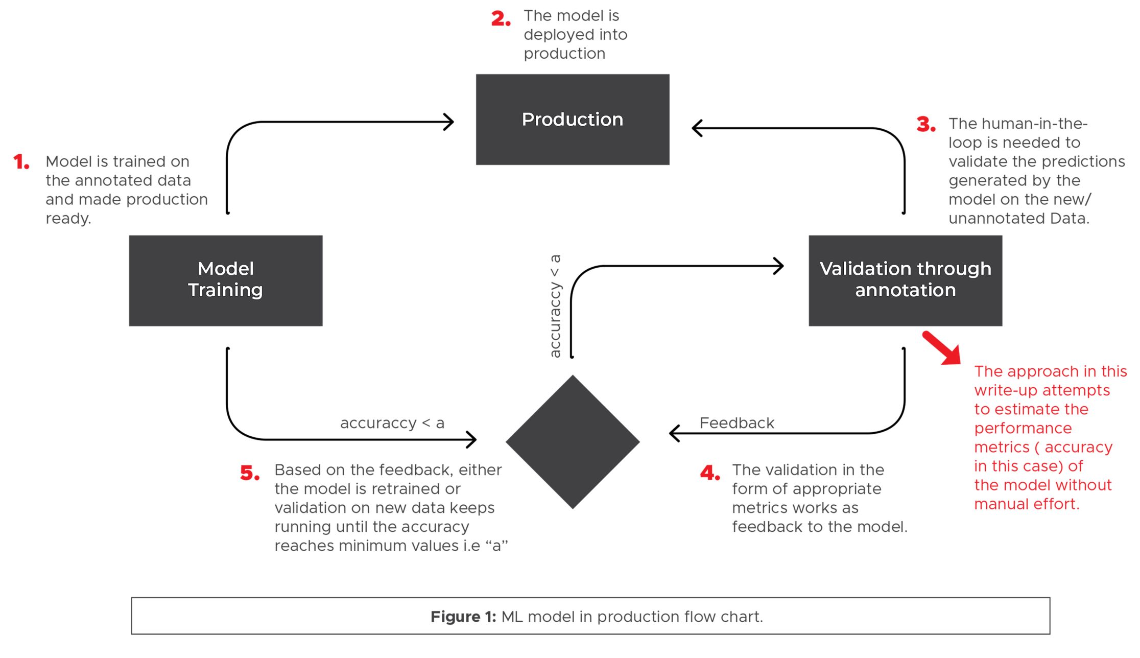
Validating a model is a crucial step in the machine learning pipeline. It helps to assess the performance and reliability of a trained model on unseen data. Validation allows us to determine whether the model has learned patterns that can generalize well to new data or if it is overfitting the training data.
There are various techniques available for validating machine learning models, each with its own advantages and use cases. These techniques help to estimate the model’s performance and provide insights into its generalization capabilities, allowing us to make more informed decisions when deploying the model in real-world scenarios.
In this article, we will explore different methods of model validation, ranging from simple train-test splits to more advanced techniques like cross-validation and bootstrapping. We will also discuss commonly used performance metrics to assess the model’s accuracy, precision, recall, and other evaluation metrics.
The main goal of model validation is to ensure that the trained model will perform well on new, unseen data. By evaluating a model’s performance using different validation techniques, we can gain insights into its strengths and weaknesses. This knowledge can help us fine-tune the model and improve its predictions, leading to better outcomes in various domains such as finance, healthcare, marketing, and more.
As you continue reading, you will learn about different model validation techniques and how they can be applied to different scenarios. It is important to note that there is no one-size-fits-all approach to validation. The choice of technique depends on the nature of the data, the problem at hand, and the available resources. Therefore, it is essential to have a solid understanding of these methods to select the most appropriate approach for your specific machine learning task.
Cross-Validation
Cross-validation is a widely used model validation technique that helps to estimate the performance of a model by partitioning the data into multiple sets and iteratively training and testing the model on different combinations of these sets.
The most common form of cross-validation is the k-fold cross-validation, where the data is divided into k equally sized folds. The model is then trained on k-1 folds and tested on the remaining fold. This process is repeated k times, with each fold serving as the test set once. The performance metrics are then averaged over all iterations to obtain an overall estimation of the model’s performance.
K-fold cross-validation provides a more reliable estimate of the model’s performance compared to a single train-test split. It helps to reduce the bias that can arise from using only one specific split and provides a better representation of the model’s generalization capabilities.
Another variation of k-fold cross-validation is stratified k-fold cross-validation. This technique ensures that each fold contains a proportional representation of each class in the dataset. It is particularly useful when dealing with imbalanced datasets where some classes have a smaller number of samples.
Leave-one-out cross-validation (LOOCV) is a special case of k-fold cross-validation where k is equal to the number of samples in the dataset. In each iteration, the model is trained on all but one sample and tested on the left-out sample. This is a computationally expensive technique, but it provides an unbiased estimate of the model’s performance.
For larger datasets, repeated k-fold cross-validation can be used. This technique randomly splits the data into k folds multiple times and averages the performance metrics over these iterations. It helps to increase the robustness of the estimation and reduces the variability that can arise from a single split.
Cross-validation is particularly useful when dealing with limited data. It allows us to make the most efficient use of the available samples and provides a more accurate evaluation of the model’s performance. By using cross-validation, we can identify and address overfitting or underfitting issues, choose the best hyperparameters, and have a more realistic understanding of the model’s behavior on unseen data.
Train-Test Split
The train-test split is one of the simplest methods for model validation. It involves dividing the dataset into two parts: a training set and a testing (or validation) set. The model is trained on the training set and evaluated on the testing set to assess its performance.
The train-test split is typically performed using a random sampling technique, where a certain percentage of the data is allocated to the training set, and the remaining data is assigned to the testing set. The ratio of the split depends on the size of the dataset and the specific requirements of the problem at hand. A common practice is to allocate around 70-80% of the data for training and the rest for testing.
The training set is used to fit the model, adjusting its parameters and learning the underlying patterns and relationships in the data. This allows the model to capture the dependencies and make predictions based on the learned information. The testing set, on the other hand, is used to evaluate the performance of the trained model. It serves as an approximation of how the model will perform on unseen data.
By evaluating the model on the testing set, we can assess its ability to generalize and make accurate predictions on new, unseen data. If the model performs well on the testing set, it suggests that it has learned the patterns and can make reliable predictions. However, if the model performs poorly on the testing set, it indicates that it may be overfitting the training data or failing to capture the underlying patterns.
It is important to note that the train-test split has some limitations. It provides a single estimate of the model’s performance, which can be sensitive to the specific split of the data. In other words, the performance of the model can vary depending on which samples are included in the training and testing sets. To overcome this limitation, it is recommended to perform multiple train-test splits and average the performance metrics over these iterations.
The train-test split is a straightforward and fast validation technique that can provide initial insights into the model’s performance. It is commonly used in the early stages of model development. However, for more robust and accurate validation, more advanced techniques like cross-validation should be employed.
K-Fold Cross-Validation
K-fold cross-validation is a commonly used model validation technique that provides a more reliable estimate of a model’s performance compared to a single train-test split. It involves dividing the dataset into k equally sized folds, where k is typically a value between 5 and 10.
In each iteration of k-fold cross-validation, the model is trained on k-1 folds and tested on the remaining fold. This process is repeated k times, with each fold serving as the test set once. The performance metrics are then averaged over all iterations to obtain an overall estimate of the model’s performance.
K-fold cross-validation helps to address the issue of bias that can arise from using only one specific train-test split. By training and testing the model on different combinations of the folds, it provides a more stable and representative evaluation of the model’s generalization capabilities.
One advantage of k-fold cross-validation is that it allows for the efficient use of data. Each sample in the dataset has the opportunity to be part of the training set as well as the testing set. This is especially useful when dealing with limited data, as it maximizes the information utilized for model validation.
As mentioned earlier, for larger datasets, it is common to use lower values of k, such as 5 or 10. On the other hand, for smaller datasets, higher values of k, such as 10 or even 20, may provide a more accurate estimate of the model’s performance.
One variation of k-fold cross-validation is stratified k-fold cross-validation. This technique ensures that each fold contains a proportional representation of each class in the dataset. It is particularly useful when dealing with imbalanced datasets where some classes have a smaller number of samples.
K-fold cross-validation is a widely employed technique for model validation due to its effectiveness in estimating the performance of a model. It helps in identifying and addressing issues like overfitting or underfitting, selecting the best hyperparameters for the model, and providing a more realistic understanding of how the model will perform on unseen data.
Stratified K-Fold Cross-Validation
Stratified k-fold cross-validation is a variation of k-fold cross-validation that ensures an equal representation of each class in the dataset within each fold. This technique is particularly useful when dealing with imbalanced datasets, where some classes may have a disproportionately small number of samples.
In regular k-fold cross-validation, the data is split into k folds randomly, which may result in some folds having a significantly different distribution of classes than others. This can lead to biased performance estimates, especially if the class distribution is imbalanced.
Stratified k-fold cross-validation addresses this issue by aiming for a proportional representation of each class in each fold. It preserves the overall class distribution in the dataset while splitting it into folds for training and testing.
The process of performing stratified k-fold cross-validation is similar to regular k-fold cross-validation. The dataset is first divided into k equally sized folds. Then, in each iteration, the model is trained on k-1 folds (with the proportional class distribution preserved) and tested on the remaining fold.
The advantages of stratified k-fold cross-validation are twofold. First, it provides a more accurate assessment of the model’s performance on individual classes, ensuring that the performance estimates are not biased by the class distribution. Second, it helps in evaluating how well the model generalizes across all classes, giving a more comprehensive understanding of its overall performance.
Stratified k-fold cross-validation is commonly used in classification tasks where maintaining the balance of class representation is crucial. By using this technique, researchers and practitioners can obtain more reliable and unbiased performance estimates for their models, especially in scenarios involving imbalanced datasets.
It’s important to note that stratified k-fold cross-validation can require additional computational resources compared to regular k-fold cross-validation, as extra steps are involved in preserving the class distribution. However, the improved estimation of model performance on imbalanced datasets makes it a valuable technique in machine learning validation.
Leave-One-Out Cross-Validation
Leave-One-Out Cross-Validation (LOOCV) is a special case of k-fold cross-validation where k is equal to the number of samples in the dataset. It is an exhaustive cross-validation technique that provides an unbiased estimate of the performance of a model.
In each iteration of LOOCV, the model is trained on all but one sample and tested on the left-out sample. This process is repeated for every sample in the dataset, resulting in a sequence of model fits and evaluations. The performance metrics obtained from each iteration are then averaged to obtain the overall estimate of the model’s performance.
LOOCV is particularly useful when dealing with small datasets, as it maximizes the use of available data for both training and testing. It allows each sample to serve as a test set once, ensuring that every sample contributes to the evaluation of the model’s performance.
One advantage of LOOCV is that it provides an unbiased estimate of the model’s performance. Since each sample is tested individually, the evaluation is not influenced by the specific combination of training and testing samples as in other cross-validation techniques. This makes LOOCV a reliable method for estimating the model’s accuracy and generalizability.
However, LOOCV can be computationally expensive, especially for large datasets. The number of iterations required is equal to the number of samples in the dataset, which can be time-consuming for complex models or large datasets. As a result, LOOCV may not be feasible in all situations, and other variations of cross-validation, such as k-fold cross-validation, may be more practical.
LOOCV is commonly used in situations where every sample is valuable and the dataset size is small. It provides a comprehensive evaluation of the model’s performance by testing it on all possible combinations of training and testing samples. Moreover, LOOCV is widely employed in benchmarking studies and when comparing different models or algorithms.
Overall, LOOCV is a powerful cross-validation technique that ensures an unbiased assessment of model performance. Its exhaustive nature contributes to a thorough evaluation of the model’s capabilities, especially in scenarios where the dataset is limited in size.
Repeated K-Fold Cross-Validation
Repeated K-Fold Cross-Validation is a technique used to increase the robustness and reliability of the validation process. It is an extension of the traditional K-fold cross-validation method where the process is repeated multiple times.
Regular K-fold cross-validation splits the dataset into K equally sized folds and performs the training and testing steps for each fold. Repeated K-fold cross-validation takes this a step further by repeating the entire K-fold process multiple times, each with a new random partitioning of the dataset.
The goal of using repeated K-fold cross-validation is to obtain a more stable estimate of the model’s performance by averaging the results over multiple iterations. This helps to reduce the variability that can arise from a single split and provides a more reliable assessment of the model’s generalization ability.
One advantage of repeated K-fold cross-validation is that it allows for a more comprehensive evaluation of the model’s performance. By repeating the cross-validation process, different combinations of training and testing samples are generated, providing a richer assessment of the model’s behavior on different subsets of the data.
The number of repetitions in repeated K-fold cross-validation can vary depending on the dataset size and the level of confidence desired in the performance estimation. Common practice suggests repeating the process 5 to 10 times, but this can be adjusted based on individual requirements.
It is important to note that repeated K-fold cross-validation can be computationally more expensive compared to regular K-fold cross-validation due to the increased number of iterations. However, the additional computation time pays off by providing a more robust evaluation of the model’s performance.
Repeated K-fold cross-validation is especially beneficial when working with smaller datasets or when there is a need for a more stable estimate of the model’s accuracy. It helps to account for the random variations in the performance metrics that can occur due to the specific subsets of data used in the cross-validation process.
By using repeated K-fold cross-validation, researchers and practitioners can obtain more reliable and robust estimates of the model’s performance. This, in turn, allows for better decision-making in terms of model selection, hyperparameter tuning, and understanding the model’s behavior on unseen data.
Time Series Cross-Validation
Time Series Cross-Validation is a validation technique specifically designed for time series data, where the temporal order of the data points is important. Unlike other validation methods, such as K-fold cross-validation, time series cross-validation takes into account the chronological nature of the data.
In time series cross-validation, the dataset is split into sequential blocks, where each block represents a period of time. The model is then trained on data from earlier blocks and tested on data from later blocks. This mimics the real-world scenario where the model is exposed to historical data and evaluated based on its ability to make accurate predictions on future data.
A common approach to time series cross-validation is called rolling-window cross-validation. In this method, a fixed-size window moves across the dataset, and the model is trained on the data within the window and tested on the next data point outside the window. This process continues until the end of the dataset is reached, providing multiple evaluation points throughout the time series.
Another technique used in time series cross-validation is expanding window cross-validation. In this method, the training set starts with the initial block of data, and the testing set gradually expands with each iteration. This allows the model to be tested on progressively more recent data as the training set grows.
Time series cross-validation is essential for accurately evaluating the performance of models on time-dependent data and making predictions in a real-world setting. It helps to assess the model’s ability to capture temporal patterns, identify seasonality or trends, and handle any changing patterns over time.
One challenge in time series cross-validation is ensuring that the training set comes before the testing set in terms of chronological order. This is important to simulate the real-world scenario where the model cannot use future information to predict the past. Care should also be taken to handle any seasonality or trends in the data when splitting it into blocks during cross-validation.
By using time series cross-validation, practitioners can gain a better understanding of how well their models perform in predicting future values and detecting patterns in time series data. This technique is especially valuable in domains such as finance, weather forecasting, and stock market analysis, where historical trends and patterns play a crucial role in making accurate predictions.
Bootstrapping
Bootstrapping is a resampling technique used for estimating the variability of a model’s performance or statistical measures by creating multiple pseudo-datasets from the original data. It is particularly useful when the dataset is limited or when there is a need to obtain more reliable estimates without relying on assumptions about the underlying data distribution.
The bootstrapping process involves random sampling with replacement. From the original dataset, multiple pseudo-datasets of the same size are created by randomly selecting samples with replacement. This means that each pseudo-dataset can contain duplicates of the original samples, while some samples might not be selected at all.
Each pseudo-dataset is then used to train and test the model, and the performance metrics of interest (such as accuracy, mean squared error, or confidence intervals) are computed. By repeating this process multiple times, typically a few hundred or thousand iterations, a distribution of the performance metrics can be obtained.
Bootstrapping allows for a robust estimation of the model’s performance by taking into account potential variability in the data. It helps to quantify the uncertainty associated with the performance metrics and provides insight into the stability and reliability of the model’s predictions.
One advantage of bootstrapping is that it can be used to generate confidence intervals for the performance measures. These intervals reflect the range within which the true performance of the model is likely to fall, given the available data. The confidence intervals provide a measure of the uncertainty associated with the performance estimation and can be used for hypothesis testing or model selection.
Bootstrapping is not limited to model performance evaluation but can also be applied to other statistical measures, such as parameter estimation or feature importance ranking. It allows for a comprehensive assessment of a model’s behavior and aids in decision-making regarding the model’s reliability and suitability for the given problem.
While bootstrapping is a powerful tool, it is important to strike a balance between the number of pseudosdatasets created and computational resources. Generating too few pseudo-datasets may result in imprecise estimates, while generating too many can lead to excessive computational overhead.
Overall, bootstrapping is a valuable technique for model validation and estimating the variability of performance measures. By providing a more comprehensive understanding of a model’s behavior, it assists researchers and practitioners in making informed decisions about the model’s performance and reliability.
Performance Metrics for Model Validation
Performance metrics are essential tools for evaluating the effectiveness and accuracy of a model during the validation process. These metrics provide quantitative measures of how well the model is performing and help to assess its suitability for the given task. The choice of performance metrics depends on the specific problem domain and the desired outcome. In this section, we will discuss some commonly used performance metrics for model validation.
1. Accuracy: Accuracy measures the proportion of correct predictions made by the model among all the predictions. It is widely used for classification tasks and provides a general overview of the model’s performance.
2. Precision and Recall: Precision and recall are metrics commonly used in binary classification tasks. Precision measures the proportion of true positive predictions among all positive predictions, while recall measures the proportion of true positive predictions among all actual positive instances. These metrics are particularly useful when dealing with imbalanced datasets.
3. F1 Score: The F1 score is the harmonic mean of precision and recall. It provides a single metric that balances both precision and recall, offering a more comprehensive evaluation of the model’s performance.
4. Mean Squared Error (MSE): MSE measures the average squared difference between the predicted values and the actual values. It is commonly used for regression tasks and provides an indication of the model’s ability to estimate continuous numerical values.
5. R-squared (R²): This metric measures the proportion of variance in the dependent variable that is explained by the model. It ranges from 0 to 1, with 1 indicating a perfect fit. R-squared is often used to assess the goodness of fit in regression tasks.
6. Area Under the Curve (AUC): AUC is typically used in binary classification tasks to evaluate the performance of a model’s receiver operating characteristic (ROC) curve. It provides an aggregate measure of the model’s discriminative power and is particularly useful when the class distribution is imbalanced.
7. Mean Average Precision (mAP): mAP is commonly used in object detection or information retrieval tasks. It measures the average precision of the model across multiple classes or queries, providing a comprehensive evaluation of the model’s performance.
8. Cross-Entropy Loss: Cross-entropy loss is often used as a performance metric in multi-class classification tasks where the outputs are probabilities. It quantifies the difference between the predicted class probabilities and the true class probabilities.
It’s important to carefully select the appropriate performance metric(s) that align with the specific goals and requirements of the problem at hand. Additionally, it is common to consider multiple metrics together to gain a more holistic understanding of the model’s strengths and weaknesses.
Conclusion
Model validation is a critical step in the machine learning pipeline that ensures the reliability and generalizability of trained models. Through various validation techniques such as cross-validation, train-test split, bootstrapping, and time series cross-validation, we can evaluate a model’s performance, identify overfitting or underfitting issues, and make informed decisions about its deployment in real-world scenarios.
Each validation technique offers unique advantages and should be chosen based on the specific requirements of the problem at hand. Cross-validation, with its variations like k-fold cross-validation, stratified k-fold cross-validation, and leave-one-out cross-validation, provides more reliable performance estimates by using multiple splits of the data and accounting for imbalanced datasets or limited sample sizes.
Train-test splits offer a simple and quick way to evaluate a model’s performance, while bootstrapping allows for robust estimation of performance measures and the quantification of uncertainty. Time series cross-validation takes into account the temporal nature of data, facilitating accurate evaluation of models in predicting future values and detecting patterns over time.
To assess the effectiveness and accuracy of models, various performance metrics such as accuracy, precision, recall, F1 score, mean squared error, R-squared, AUC, and cross-entropy loss can be utilized. It is crucial to choose the appropriate metrics based on the problem domain and objectives, considering factors like class imbalance, continuous numerical values, or multi-class classification.
By employing these validation techniques and performance metrics, researchers and practitioners can gain insights into a model’s behavior, select the best-performing model, and fine-tune its hyperparameters. This ultimately helps in building reliable, accurate, and robust machine learning models that can be confidently deployed in real-world applications.
As the field of machine learning continues to evolve, further advancements and techniques in model validation will emerge. Staying informed about the latest practices and methodologies is key to ensuring the continued improvement and effectiveness of machine learning models in solving complex problems across diverse domains.


