Introduction
Google Sheets is a powerful online spreadsheet tool that allows users to organize, analyze, and calculate data. One of the most commonly used functions in Google Sheets is the SUM function, which allows you to add up the values in a range of cells. Whether you’re trying to calculate a simple sum or perform more advanced calculations with criteria, Google Sheets has got you covered.
Whether you’re new to Google Sheets or looking to expand your spreadsheet skills, this guide will walk you through the basics of using the SUM function. You’ll learn how to add individual cells, a range of cells, and even how to ignore errors in your calculations. Additionally, we’ll explore how to use the SUMIF and SUMIFS functions to perform calculations based on specific criteria.
This guide assumes that you have a basic understanding of how to use Google Sheets and that you have a spreadsheet open that you would like to perform calculations on. So let’s jump right in and explore the various ways to use the SUM function in Google Sheets.
Getting Started
Before we dive into the specifics of using the SUM function in Google Sheets, let’s first make sure you have a solid foundation to work from. If you haven’t done so already, open up a new or existing Google Sheets document and follow along with the steps below:
- Open Google Sheets: Open your preferred web browser, navigate to Google Sheets, and sign in to your Google account.
- Create a New Spreadsheet: Click on the “+ New” button to create a new spreadsheet, or select an existing spreadsheet from your Google Drive.
- Add Data: Enter some sample data into your spreadsheet. For example, you can input numbers into different cells, such as A1, A2, A3, and so on.
Once you have your spreadsheet set up with data, you’re ready to start using the SUM function to perform calculations. Now let’s move on to the next section to learn how to use the SUM function in Google Sheets.
Using the SUM function
The SUM function in Google Sheets is a simple yet powerful tool that allows you to quickly calculate the sum of a range of cells. To use the SUM function, follow these steps:
- Select a cell where you want the sum to appear. This can be any empty cell in your spreadsheet.
- Type the equal sign (=) followed by the word “SUM”.
- Open parenthesis “(” to indicate the beginning of the function.
- Select the first cell of the range you want to add.
- If you want to add more cells to the range, separate them with commas.
- Close the parenthesis “)” to indicate the end of the function.
- Press Enter to calculate the sum.
For example, if you want to add the values in cells A1, A2, and A3, you would enter the following formula: “=SUM(A1,A2,A3)”. The result will be displayed in the cell where you entered the formula.
Alternatively, you can also use the colon (:) to specify a range of cells. For example, to add the values in cells A1 to A3, you would enter the formula “=SUM(A1:A3)”. This is a convenient way to calculate the sum of a large range of cells without having to list them individually.
Now that you know how to use the SUM function, let’s move on to the next section to learn how to add multiple cells using the SUM function.
Adding multiple cells
When using the SUM function in Google Sheets, you can easily add multiple cells by specifying each cell individually as arguments within the function. This allows you to perform calculations on non-contiguous cells or select specific cells that you want to include in the sum.
To add multiple cells using the SUM function, follow these steps:
- Select a cell where you want the sum to appear.
- Type the equal sign (=) followed by the word “SUM”.
- Open parenthesis “(” to indicate the beginning of the function.
- Select the first cell you want to add.
- If you want to add more cells, separate them with commas.
- Close the parenthesis “)” to indicate the end of the function.
- Press Enter to calculate the sum.
For example, if you want to add the values in cells A1, B2, and C3, you would enter the following formula: “=SUM(A1, B2, C3)”. The result will be displayed in the cell where you entered the formula.
You can continue adding more cells by simply separating them with commas. For instance, “=SUM(A1, B2, C3, D4)” will calculate the sum of the values in cells A1, B2, C3, and D4.
This flexibility allows you to add specific cells from different parts of your spreadsheet without needing to define a range. It enables you to perform calculations based on your specific needs and requirements.
Now that you know how to add multiple cells using the SUM function, let’s move on to the next section to learn how to add a range of cells.
Adding a range of cells
Another useful feature of the SUM function in Google Sheets is the ability to add a range of cells. This allows you to easily calculate the sum of a continuous series of cells without having to specify each cell individually.
To add a range of cells using the SUM function, follow these steps:
- Select a cell where you want the sum to appear.
- Type the equal sign (=) followed by the word “SUM”.
- Open parenthesis “(” to indicate the beginning of the function.
- Select the starting cell of the range you want to add.
- Type a colon (:) to indicate the range.
- Select the ending cell of the range you want to add.
- Close the parenthesis “)” to indicate the end of the function.
- Press Enter to calculate the sum.
For example, if you want to add the values in cells A1 to A5, you would enter the formula “=SUM(A1:A5)”. The result will be displayed in the cell where you entered the formula.
This method is particularly useful when you have a large range of cells that you want to include in your calculation. Instead of writing each cell reference manually, you only need to specify the starting and ending cells, separated by a colon. Google Sheets will automatically calculate the sum of all the cells within that range.
Now that you know how to add a range of cells using the SUM function, let’s move on to the next section to learn how to ignore errors in your calculations.
Ignoring errors
When working with data in Google Sheets, you may encounter errors such as #VALUE!, #DIV/0!, or #REF!, which can disrupt your calculations. However, you can instruct the SUM function to ignore these errors and still perform the sum on the valid cells within a range.
To ignore errors when using the SUM function, you can utilize the IFERROR function as a wrapper around the SUM function. Here’s how you can do it:
- Select a cell where you want the sum to appear.
- Type the equal sign (=) followed by the word “IFERROR”.
- Open parenthesis “(“.
- Inside the IFERROR function, type the SUM function along with the range of cells you want to add.
- Close the parenthesis “)” for the SUM function.
- After the closing parenthesis, type a comma (,) followed by 0 or any other desired value to display in case of an error.
- Close the parenthesis “)” for the IFERROR function.
- Press Enter to calculate the sum.
When an error is encountered within the range, the IFERROR function will return the value specified after the comma, which can be 0 or any other desired output. This ensures that your sum calculation is not disrupted by the presence of errors.
For example, if you have a range of cells A1 to A4, but cell A3 contains an error, you can use the following formula: “=IFERROR(SUM(A1:A4), 0)”. This formula will calculate the sum of cells A1, A2, and A4 while ignoring the error in cell A3.
By incorporating the IFERROR function, you can enhance the accuracy and reliability of your calculations, even when dealing with potentially faulty data.
Now that you know how to ignore errors in your calculations, let’s move on to the next section to learn how to use criteria with the SUMIF function.
Using criteria with SUMIF
The SUMIF function in Google Sheets allows you to calculate the sum of a range of cells based on a specific criteria. This function is particularly helpful when you want to perform calculations on data that meets certain conditions.
To use the SUMIF function, follow these steps:
- Select a cell where you want the sum to appear.
- Type the equal sign (=) followed by the word “SUMIF”.
- Open parenthesis “(” to indicate the beginning of the function.
- Select the range of cells that you want to evaluate for the criteria.
- Type a comma (,) to separate the range from the criteria.
- Enter the criteria within quotation marks (“”) or reference a cell that contains the criteria.
- If you want to add a specific range of cells that meet the criteria, select the range. Otherwise, use the entire range.
- Close the parenthesis “)” to indicate the end of the function.
- Press Enter to calculate the sum based on the specified criteria.
For example, let’s say you have a list of sales amounts in column A and you want to calculate the sum of all values that are greater than $100. You would enter the formula “=SUMIF(A:A, “>100″)”. This formula will add up all the values in column A that meet the criteria of being greater than $100.
The SUMIF function allows you to perform calculations based on various criteria such as text, numbers, or logical expressions. Experiment with different criteria to customize your calculations according to your specific data and requirements.
Now that you know how to use criteria with the SUMIF function, let’s move on to the next section to learn how to use multiple criteria with the SUMIFS function.
Using multiple criteria with SUMIFS
If you need to perform calculations based on multiple criteria, you can use the SUMIFS function in Google Sheets. The SUMIFS function allows you to add up values in a range of cells that meet multiple conditions simultaneously.
To use the SUMIFS function, follow these steps:
- Select a cell where you want the sum to appear.
- Type the equal sign (=) followed by the word “SUMIFS”.
- Open parenthesis “(” to indicate the beginning of the function.
- Select the range of cells that you want to evaluate for the first criteria.
- Type a comma (,) to separate the range from the first criteria.
- Select the range of cells that you want to evaluate for the second criteria.
- Type another comma (,) to separate the second criteria.
- Enter the first criteria range and criteria within quotation marks (“”) or reference a cell that contains the criteria.
- Type a comma (,) to separate the first and second criteria.
- Enter the second criteria range and criteria within quotation marks (“”) or reference a cell that contains the criteria.
- Continue this pattern if you have additional criteria to include.
- Close the parenthesis “)” to indicate the end of the function.
- Press Enter to calculate the sum based on the specified multiple criteria.
For example, suppose you have a sales table with sales amounts in column A, regions in column B, and months in column C. If you want to calculate the sum of sales amounts for the region “North” in the month of “January”, you would enter the formula “=SUMIFS(A:A, B:B, “North”, C:C, “January”)”. This formula will add up all the sales amounts that meet both criteria simultaneously.
The SUMIFS function provides a powerful way to analyze data based on multiple conditions. It allows you to filter and segment your data to extract specific information and perform targeted calculations.
Now that you know how to use multiple criteria with the SUMIFS function, you can apply this knowledge to analyze and manipulate your data in Google Sheets.
Conclusion
The SUM function in Google Sheets is a valuable tool for performing calculations on numerical data. Whether you need to add individual cells, a range of cells, or apply specific criteria, the SUM function provides an efficient way to perform these calculations.
In this guide, we have covered the basics of using the SUM function, including adding multiple cells and adding a range of cells. We have also explored how to ignore errors in your calculations and how to use criteria with the SUMIF and SUMIFS functions to perform calculations based on specific conditions.
By mastering the SUM function and its variations, you can efficiently analyze and manipulate your data in Google Sheets. Whether you’re a student, a professional, or a data enthusiast, understanding how to use the SUM function will enable you to make better sense of your data and make informed decisions.
Remember to consider the context of your data and choose the appropriate method for your calculations. Experiment with different criteria and ranges to customize your formulas and obtain the desired results. The flexibility and power of the SUM function make it an essential tool for anyone working with numbers in Google Sheets.
Now that you are equipped with the knowledge of using the SUM function in Google Sheets, go ahead and explore its capabilities. Dive into your spreadsheets, perform calculations, and uncover valuable insights within your data.