How To Add The Sum Of A Column In Google Sheets

Introduction

Welcome to this article on how to add the sum of a column in Google Sheets. Google Sheets is a powerful spreadsheet tool that allows you to perform various calculations and analysis on your data. Adding the sum of a column is a common task when working with data, whether it’s calculating sales totals, expenses, or any other numerical values.

In this step-by-step guide, we will walk you through the process of adding the sum of a column in Google Sheets. You don’t need to be an expert in spreadsheets to follow along – we will explain each step in a straightforward manner, making it easy for beginners and experienced users alike.

By the end of this article, you will have the knowledge and skills to quickly and accurately calculate the sum of a column in Google Sheets, saving you time and effort in your data analysis tasks.

So, let’s get started with the first step – opening Google Sheets.

Step 1: Open Google Sheets

The first step to adding the sum of a column in Google Sheets is to open the application. Google Sheets can be accessed through your web browser by navigating to https://www.google.com/sheets.

If you already have a Google account, simply sign in with your credentials. If you don’t have an account, you can create one for free by clicking on the “Create account” button.

Once you are signed in, you will be taken to the Google Sheets homepage where you can create a new spreadsheet or open an existing one. To create a new spreadsheet, click on the “Blank” option or select a template that suits your needs.

After selecting your desired option, Google Sheets will open, and you will be ready to start working on your spreadsheet.

Opening Google Sheets is the first and fundamental step in adding the sum of a column. Now that we have the application open, let’s move on to the next step – selecting the column to be summed.

Step 2: Select the Column to be Summed

Once you have your Google Sheets spreadsheet open, you need to select the column that you want to calculate the sum for. To do this, position your cursor in the cell of the column you wish to select.

If you want to select a single column, click on the column letter at the top of the spreadsheet. For example, if you want to sum column A, click on the letter “A”. The entire column will be highlighted to indicate that it is selected.

If you want to select multiple columns, hold down the Ctrl key (Command key on Mac) and click on the letters of the columns you want to select. For instance, if you want to sum columns A and B, click on both the letter “A” and the letter “B”. The selected columns will be highlighted.

If your data has headers, you may want to exclude the header row from the selection. To do this, click on the first cell of the column you want to sum (excluding the header), hold down the Shift key, and click on the last cell of the column. This will select the range of cells in the column, excluding the header.

By selecting the appropriate column, you ensure that only the desired data will be included in the sum calculation. With the column selected, you are now ready to move on to the next step – using the SUM function.

Step 3: Use the SUM function

Now that you have selected the column to be summed, it’s time to use the SUM function in Google Sheets to calculate the total sum. The SUM function is a built-in formula that adds up all the values in a given range.

To use the SUM function, click on the cell where you want the sum to be displayed. Then, type an equal sign (=) followed by the word “SUM” and an opening parenthesis (. For example, if you want the sum to be displayed in cell C1, you would enter “=SUM(“.

Now, select the range of cells that you want to include in the sum calculation. This can be the entire column you selected in the previous step or a specific range within that column. For example, if you selected column A, you can enter “A:A” to include the entire column, or you can enter “A1:A10” to include only cells A1 to A10.

After selecting the range, close the parenthesis ) and press Enter. The SUM function will calculate the sum of the selected range and display the result in the cell.

If you have multiple columns that you want to sum, you can use the SUM function for each column separately. For example, to calculate the sum of column A and column B, you would use the formula “=SUM(A:A) + SUM(B:B)”. The result will be the sum of the values in both columns.

Using the SUM function allows you to easily calculate the sum of a column or multiple columns in Google Sheets. With the sum calculated, you can now proceed to the next step – formatting the sum result to your desired format.

Step 4: Calculate the Sum using AutoSum

In addition to manually using the SUM function, Google Sheets provides an easy and quick way to calculate the sum using the AutoSum feature. AutoSum automatically detects the range of cells to be summed, saving you time and effort.

To use AutoSum, follow these steps:

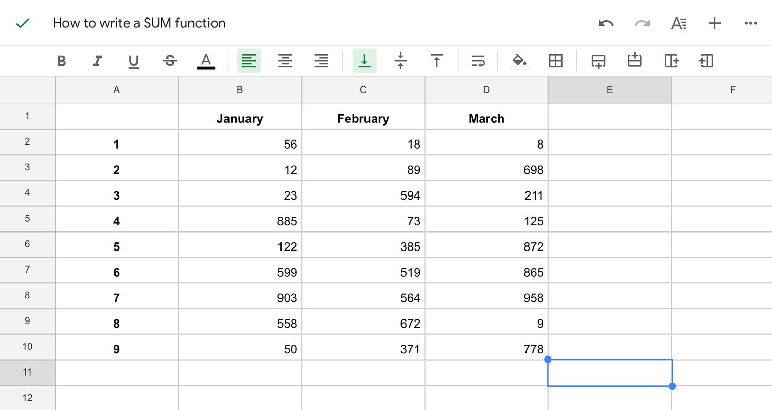
1. Select the cell where you want the sum to be displayed.
2. Click on the “Σ” symbol in the toolbar, which represents the AutoSum feature.
3. Google Sheets will automatically detect the range of cells above the selected cell, and a bounding box will appear around the range.
4. If the detected range is not what you intended to sum, you can click and drag to adjust the range manually.
5. Once you are satisfied with the range, press Enter to calculate the sum and display the result in the selected cell.

The AutoSum feature is especially useful when you have a large dataset and don’t want to manually select the range for the sum. It saves time and eliminates the possibility of selecting the wrong range by automatically detecting the appropriate cells.

Now that you have learned how to calculate the sum using AutoSum, you can move on to the next step – formatting the sum result to your desired format.

Step 5: Format the Sum Result as Desired

After calculating the sum of a column in Google Sheets, you may want to format the sum result to your desired format. Formatting the sum result can help improve the readability and visual appeal of your spreadsheet.

To format the sum result, follow these steps:

1. Select the cell containing the sum result.
2. Right-click on the cell and choose the “Format cells” option from the context menu.
3. In the Format Cells dialog box, you can customize the formatting options, such as the number format, font style, cell borders, background color, and more.
4. Choose the formatting options that suit your preferences and click “Apply” or “OK” to save the changes.

For example, you might want to format the sum result as currency with two decimal places, or you might want to apply a specific font color or background color to make it stand out.

Customizing the formatting of the sum result allows you to present your data in a visually appealing and meaningful way. Experiment with different formatting options to find the style that best fits your needs.

With the sum result formatted as desired, you have successfully completed this step. Now, let’s move on to the next step – adding the sum of multiple columns.

Step 6: Add a Sum of Multiple Columns

In addition to adding the sum of a single column, Google Sheets allows you to easily calculate the sum of multiple columns. This can be useful when you want to analyze data that spans across different columns.

To add a sum of multiple columns, follow these steps:

1. Select the cell where you want the sum of multiple columns to be displayed.
2. Enter the SUM function by typing an equal sign (=) followed by the word “SUM” and an opening parenthesis (.
3. Select the range for the first column you want to include in the sum calculation. For example, if you want to sum column A, enter “A:A”.
4. Insert a plus sign (+) to indicate that you want to add another column to the sum.
5. Select the range for the second column you want to include in the sum calculation. For example, if you want to sum column B, enter “B:B”.
6. Repeat this process for as many columns as you want to include in the sum calculation, separating each column with a plus sign (+).
7. Close the parenthesis ) and press Enter to calculate the sum of the selected columns and display the result in the cell.

For instance, if you want to calculate the sum of columns A, B, and C, you would enter the formula “=SUM(A:A) + SUM(B:B) + SUM(C:C)”. The result will be the sum of the values in all three columns.

By adding the sum of multiple columns, you can gain valuable insights and perform more complex calculations on your data within Google Sheets.

With the sum of multiple columns calculated, you have completed all the necessary steps. Congratulations!

Conclusion

Congratulations! You have successfully learned how to add the sum of a column in Google Sheets. This skill is invaluable when working with numerical data and allows you to quickly calculate totals and analyze information in your spreadsheets.

In this article, we covered the following steps:

1. Opening Google Sheets, which is the first step in accessing the spreadsheet application.
2. Selecting the column or columns to be summed.
3. Using the SUM function to calculate the sum manually.
4. Utilizing the AutoSum feature to automatically calculate the sum.
5. Formatting the sum result to suit your desired format.
6. Addling the sum of multiple columns to perform more complex calculations.

By following these steps, you now have the necessary skills to add the sum of a column or multiple columns in Google Sheets with ease. Whether it’s financial data, sales figures, or any other type of numerical information, you can confidently perform calculations and gain insights from your data.

Remember to explore additional features and functions available in Google Sheets to further enhance your data analysis capabilities. By leveraging the power of this versatile tool, you can unlock even more potential in your spreadsheet tasks.

So go ahead, put your newfound knowledge into practice, and start adding sums to your columns in Google Sheets. Happy calculating!