How To Compare Two Columns In Google Sheets

Introduction

Welcome to this guide on how to compare two columns in Google Sheets. Comparing columns in Google Sheets can be a useful way to find similarities or differences between two sets of data. Whether you’re working on a spreadsheet with customer information, inventory data, or any other type of data, being able to compare columns can help you identify patterns, discrepancies, or missing values.

In this article, we will explore different techniques to compare two columns in Google Sheets, ranging from basic comparison methods to using conditional formatting and functions. We will also touch on comparing multiple columns and handling empty cells. By the end of this guide, you will have the necessary tools to efficiently compare two columns and gain valuable insights from your data.

Google Sheets is a powerful tool that provides various features for data analysis. By leveraging the techniques discussed in this guide, you can save time and effort while ensuring accuracy in your data comparisons. Whether you’re a beginner or an experienced user, this article will provide step-by-step instructions and helpful tips to assist you in comparing two columns effectively.

So, let’s dive into the different methods and functions available in Google Sheets that allow us to compare columns and extract meaningful information from our data!

Basic Comparison

When comparing two columns in Google Sheets, the most straightforward method is to visually scan the data pairs manually. This method involves looking at each row in the two columns and identifying any similarities or differences. While this approach may be appropriate for smaller datasets, it can become time-consuming and prone to errors when dealing with large amounts of data.

To perform a basic comparison, follow these steps:

1. Select the first cell in the second column where you want to compare the values.
2. Enter the formula =A1=B1 and press Enter. This formula will compare the value in cell A1 with the value in cell B1 and return TRUE if they are equal or FALSE if they are not.
3. Drag the formula down to apply it to the rest of the cells in the column.

Once you have applied the formula to all the cells, you will be able to see the comparison results. The cells containing TRUE indicate where the values in the two columns match, while the cells with FALSE indicate where they differ. This method allows you to visually identify the similarities and differences in the two columns.

A useful feature in Google Sheets is the ability to filter the column based on the results of the comparison. You can filter the column to show only the rows where the comparison is TRUE or FALSE, depending on your requirements. This can help you focus on specific data points and draw insights from the comparison.

Remember that this basic comparison method works best for small datasets where you can manually review the results. If you’re dealing with a large amount of data or need to automate the comparison process, you can explore other techniques, which we will discuss in the following sections.

Comparing Two Columns Using Conditional Formatting

Google Sheets offers a powerful feature called conditional formatting that allows you to visually highlight cells based on specific conditions. You can use conditional formatting to compare two columns and identify matching or differing values.

To compare two columns using conditional formatting, follow these steps:

1. Select the entire range of the second column that you want to compare.
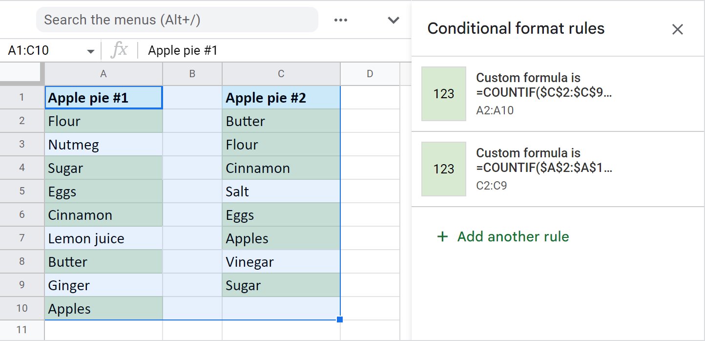
2. From the menu, go to Format > Conditional formatting.
3. In the conditional formatting rules panel, select Custom formula is from the dropdown menu.
4. Enter the formula =A:A=B:B in the input box. This formula compares each cell in column A with the corresponding cell in column B.
5. Choose the formatting options to apply to the cells that meet the specified condition. For example, you can choose to highlight the matching cells with a specific background color or add symbols.
6. Click Done to apply the conditional formatting rules.

Once you have applied the conditional formatting, Google Sheets will automatically highlight the cells that meet the specified condition. In this case, the cells that have matching values in both columns will be highlighted according to the chosen formatting options.

This technique allows you to quickly identify the matching values between the two columns and visually distinguish them from the differing values. Conditional formatting provides an efficient way to compare large datasets and draw attention to specific data points.

Furthermore, you can extend the application of conditional formatting to include additional rules based on your requirements. For example, you can add another rule to highlight cells where the values in column B are higher or lower than the corresponding values in column A.

By utilizing conditional formatting, you can easily compare two columns in Google Sheets and gain insights from the data in a visually appealing format.

Using Functions to Compare Two Columns

Google Sheets provides a range of functions that you can use to compare two columns and perform more advanced operations on the data. These functions allow you to automate the comparison process and extract valuable information from the columns.

One commonly used function for comparing two columns is the VLOOKUP function. This function helps you find the matching values in one column based on the values in another column. Here’s how you can use the VLOOKUP function:

1. In a new column, enter the VLOOKUP formula. The formula syntax is =VLOOKUP(A2, B:C, 2, false).
2. Replace A2 with the first cell reference in the first column that you want to compare.
3. Replace B:C with the range of cells containing the two columns that you want to compare. The first column should be to the left of the column you want to compare it with.
4. Specify 2 as the column index number, indicating that you want to retrieve the value from the second column of the range.
5. Set false as the last argument to ensure an exact match.

The VLOOKUP function will search for the value in the first column and return the corresponding value from the second column if there is a match. You can drag the formula down to apply it to the rest of the cells in the column. The cells will display the matching values from the second column or #N/A if there is no match.

Aside from VLOOKUP, Google Sheets includes other functions such as INDEX, MATCH, and COUNTIF that can be useful for comparing columns and performing advanced operations.

By utilizing these functions, you can streamline the comparison process and obtain valuable insights from your data. Whether you need to find matching values, identify differences, or perform calculations, using functions in Google Sheets will enhance your ability to analyze and compare two columns efficiently.

Comparing Multiple Columns

Comparing multiple columns in Google Sheets allows you to analyze and identify patterns or differences across multiple sets of data. This can be particularly useful when dealing with complex datasets or when trying to find relationships between different categories of information.

To compare multiple columns, you can use various techniques, depending on the specific requirements of your analysis. Here are a few methods:

1. Conditional Formatting: Apply conditional formatting to the range of cells that includes the multiple columns you want to compare. You can set up different rules for each column or create rules based on combinations of columns. This will allow you to visualize any similarities or differences between the columns.

2. Concatenate and Compare: Create a new column where you concatenate the values from each row of the multiple columns. Then, use the techniques discussed earlier, such as basic comparison or conditional formatting, on the concatenated column to identify matching or differing values.

3. VLOOKUP and IFNA: Use the VLOOKUP function along with the IFNA function to compare multiple columns. You can set up nested VLOOKUP functions to check for matches across multiple columns and display the result accordingly. The IFNA function allows you to handle cases where there are no matches.

4. Array Formulas: Array formulas are powerful tools that allow you to perform calculations and comparisons across multiple columns simultaneously. Using functions like ARRAYFORMULA, TRANSPOSE, and operators like = or <>, you can compare the values in different columns and retrieve the desired results.

These methods provide different ways to compare multiple columns in Google Sheets, depending on the complexity and nature of your data. Experiment with these techniques and choose the one that best suits your analysis goals.

By comparing multiple columns, you can gain a comprehensive understanding of the relationships and patterns within your data, enabling you to make informed decisions and draw valuable insights for your project or analysis.

Handling Empty Cells

When comparing columns in Google Sheets, it’s common to come across empty cells or cells with missing values. These empty cells can affect the accuracy of your comparisons, as they may lead to false matches or differences. Therefore, it’s important to handle empty cells appropriately to ensure reliable and meaningful results.

Here are a few approaches you can take to handle empty cells when comparing columns:

1. Ignore empty cells: One simple option is to ignore empty cells when performing comparisons. This means that empty cells will not be considered when checking for matches or differences. You can achieve this by using conditional formatting rules or custom formulas that exclude empty cells from the comparison.

2. Treat empty cells as a specific value: Instead of ignoring empty cells, you can choose to treat them as a specific value during the comparison. For example, you can consider empty cells as “N/A,” “Null,” or any other value that represents missing data. By assigning a specific value to empty cells, you can include them in the comparison process and account for missing information.

3. Apply conditional logic: Another approach is to use conditional logic to handle empty cells. For example, you can use functions like IF or ISBLANK to check if a cell is empty before performing a comparison. You can then define what action or value should be taken when encountering empty cells, such as skipping the comparison or assigning a specific result.

4. Data cleaning: If your dataset contains a significant number of empty cells, you may consider cleaning the data before comparing the columns. Data cleaning involves removing or filling in the empty cells with appropriate values, such as using the FILTER or IFERROR functions. By cleaning the data, you can ensure more accurate and meaningful comparisons.

When handling empty cells, it’s essential to consider the specific requirements of your analysis and the nature of your data. Each approach has its own advantages and considerations, so choose the method that aligns with your analysis goals and produces the desired results.

By appropriately handling empty cells, you can ensure the integrity of your data comparisons and obtain more accurate insights from your analysis.

Dealing with Case Sensitivity

When comparing columns in Google Sheets, you may come across situations where the comparison needs to be case-insensitive. Case sensitivity refers to whether uppercase and lowercase letters are treated as distinct values or not. By default, comparisons in Google Sheets are case-sensitive, meaning that uppercase and lowercase letters are considered different.

To deal with case sensitivity when comparing columns, you can use various techniques:

1. Convert to lowercase or uppercase: One approach is to convert the values in both columns to either lowercase or uppercase using the LOWER or UPPER function. By applying this function to each cell or to the entire column, you can standardize the cases and make the comparison case-insensitive.

2. Use the EXACT function: The EXACT function in Google Sheets performs a case-sensitive comparison between two strings. To make the comparison case-insensitive, you can use the LOWER or UPPER function in conjunction with EXACT. For example, the formula =EXACT(LOWER(A1), LOWER(B1)) will compare the values in cell A1 and B1 after converting them to lowercase.

3. Apply conditional formatting: Conditional formatting rules can be used to highlight matching or differing cells while ignoring case sensitivity. You can create custom rules using formulas that compare the lowercased or uppercased values in the columns. This way, the formatting will reflect the comparison results without being affected by different cases in the data.

4. Use the QUERY function: The QUERY function allows you to perform more advanced data manipulations and comparisons. By using the LOWER or UPPER functions within the QUERY formula, you can create case-insensitive comparisons and retrieve the desired results.

When dealing with case sensitivity, it’s important to consider the requirements of your specific analysis and determine which method suits your needs. By implementing these techniques, you can ensure accurate and comprehensive comparisons, regardless of the cases of the values in the columns.

Summary

Comparing two columns in Google Sheets is a valuable technique that allows you to gain insights, identify patterns, and analyze data effectively. With the range of tools and functions available, you can easily compare columns and extract meaningful information from your dataset.

In this guide, we explored various methods for comparing two columns in Google Sheets. We started with the basic approach of visually scanning the data pairs and then moved on to more advanced techniques, such as using conditional formatting to highlight matching values. We also discussed how to utilize functions like VLOOKUP to automate the comparison process and explore multiple columns simultaneously.

We also covered important considerations like handling empty cells and dealing with case sensitivity. By addressing these factors, you can ensure accurate and comprehensive comparisons, avoiding false matches or discrepancies caused by missing values or different cases.

Remember to choose the most suitable method based on the size and complexity of your dataset, as well as the specific requirements of your analysis. Whether you’re working with small or large datasets, manually comparing columns or using advanced functions, Google Sheets provides the tools to streamline your analysis and uncover valuable insights.

By utilizing the techniques and strategies discussed in this guide, you can enhance your data analysis skills and confidently compare two columns in Google Sheets, unlocking the full potential of your data.