In the modern world, machine learning has become an essential aspect of success both in business and research. It has an algorithm that automates every business process. In this article, we will learn about Machine Learning and we will explore different algorithms, applications, and usage of Python programming language.
For beginners, First, let’s begin with the theoretical background of Machine Learning. Machine learning is not new in computing. Instead, it is one of the fastest technology that evolves over time. In 1943, Neural networks were first introduced by mathematician Walter Pitts and Neurophysiologist Warren McCulloh. After that, in 1958, Perceptron was created as the first Artificial Neural Network. It was created by Frank Rosenblatt to recognize patterns and shapes.
Fast forward, so finally, in the 21st century with the leadership of big players such as Google, Amazon, Facebook, and others. There are more and more algorithms, research and development in this field. Thus, this encourages more and more innovation and invention in the field of computing.

What is Machine Learning?
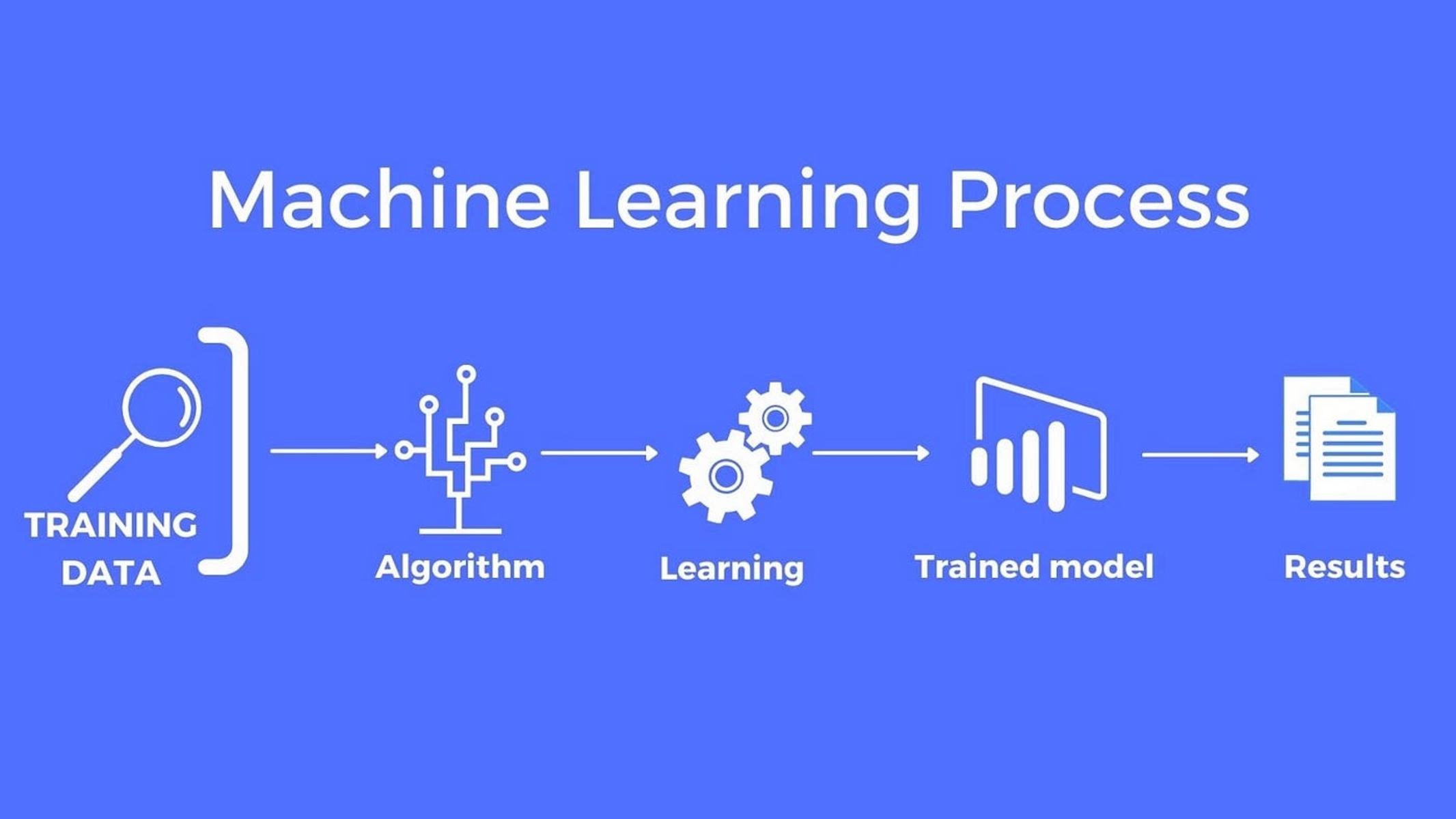
Machine learning is one of the hot topics in Artificial Intelligence where it provides computers the competence to learn without being explicitly programmed. It also has an algorithm that allows applications to have more accurate results. In addition, in predicting outcomes, it provides accurate results without being obviously programmed. Machine learning usually builds algorithms that have input data and it uses statistical analysis. It is used to predict an outcome while updating outputs as new data. Methods involved in machine learning are related to data mining and predictive modeling. The process requires searching data to find patterns and regulating actions accordingly.
One great example is when you’re using your social media accounts where it learns your browsing experience. You can notice this through the ads it appears on your account. Recommendation engines use machine learning to personalize online ads in real-time aspects. Aside from search engine recommendation, machine learning also uses for spam filtering, network detection threat and predictive maintenance.
What are the Algorithms in Machine Learning?
Talking about an algorithm, Machine learning has a lot of algorithms to explore.
These algorithms categorize into groups:
- Supervised Learning
- Unsupervised Learning
- Semi-supervised Learning
- Reinforcement Learning
When we talked about Supervised Learning, this means that the computer has the ability to recognize data based on the provided samples. A computer learns and improves the ability to understand new data based on the original data.
Algorithms under supervised learning include the following:
- Linear Regression
- Support-vector Machine(SVM)
- Decision Trees
- Naïve Bayes classifier
- K-Nearest Neighbor
Unsupervised Learning works in a way that a computer program trains with unlabeled data. The machine is the one to determine the relationship between input data and other relevant data. This indicates that the computer itself looks for patterns and relationships between the data sets. In this area of machine learning, this is very useful in pattern detection and descriptive modeling. When in cases where a human doesn’t have an idea what to look for in the data set. This algorithm doesn’t determine the right output but it explores the data. After, it can categorize inferences from datasets to describe hidden data from unlabeled data.
Under supervised learning are the following algorithms:
- K-means Clustering
- Association Rules
Due to the limitations of both supervised and unsupervised learning, Semi-supervised learning has found its way to these limitations. In other words, semi-supervised Learning descends from both supervised and unsupervised learning. For some instances, labeling data might cost high since it needs the skills of the experts. Therefore, semi-supervised learning can use as unlabeled data for training. Usually, this type of machine learning involves a small amount of labeled data and it has a large amount of unlabeled data.
Algorithms under semi-supervised learning are the following:
- Continuity Assumption
- Cluster Assumption
- Manifold Assumption
On the other hand, Reinforcement Learning is a method that allows interaction with its environment. In other words, it interacts by creating actions and discovers errors. This learning typically has a characteristic of a trial and error search and reward delays. Furthermore, this allows computers and software applications to automatically determine the behavior within a specific context to maximize its performance. Some reinforcement learning applications include robotic hands, self-driving cars, and other computer-related games.
List of the algorithm under reinforcement learning are the following:
- Temporal Difference(TD)
- Q-Learning
- Deep Adversarial Networks
How to start Machine learning in Python?
Python is one of the best programming languages to use in machine learning applications. Before we start with deeper discussions on Python, first you need to install the following tools in order to get started. Make sure to install the latest version.
List of tools you need:
- Python Programming LanguageTensorFlow
- Keras
- Shogun
- Scikit-Learn
- Theano
- NLTK
- Numpy
- Pandas
- Anaconda
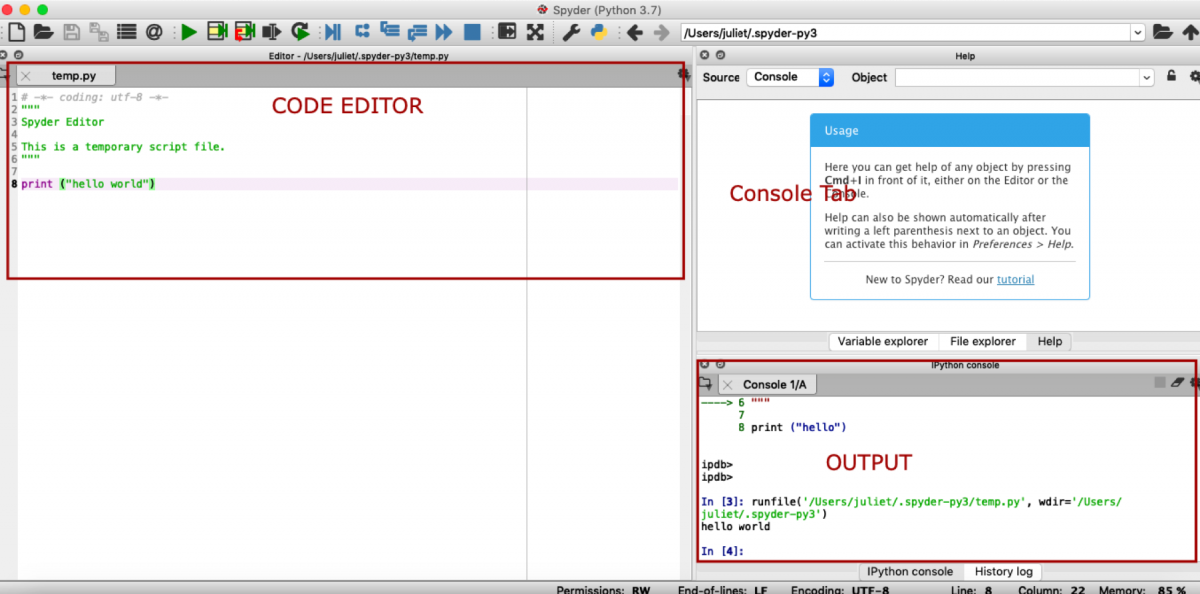
In my own preference, I only installed anaconda on my machine which is the most basic and relevant framework and IDE’s are already included. Here’s how it looks like upon opening your anaconda installed.
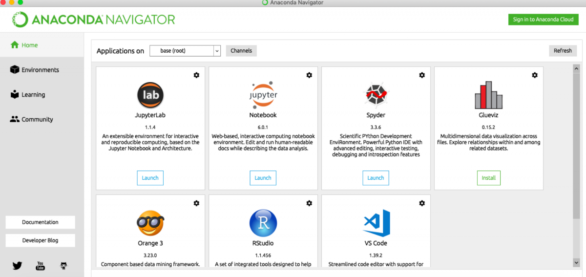
Anaconda gives you options on what kind of IDE you are going to use. In my case, I like using the Spyder IDE than others. Here’s a sample screenshot of Spyder IDE running a simple “hello world” in python.
Python’s Basic Syntax
After installing and setting up all the needed tools, Let’s start with some basics! In machine learning, there are a series of steps and processes to follow. This article will only focus on the mathematical aspect and data visualization using python. In my example below, I will be using a supervised learning algorithm.
DATA
In data science or any machine learning program, data is an essential and important ingredient in this topic. For beginners that want to explore the world of data science, you can download data from different databank or data repository. On my own preference, I downloaded some of my data from www.kaggle.com. Another option to have data is to personally collect the data needed for learning. In my example today, I downloaded data from kaggle regarding, mental health. These data are reported suicide rates from 1985 to 2016.
LIBRARIES
Python has a lot of libraries to offer for machine learning. In my sample code, I’m using the following libraries.
- Numpy is one of the primary packages in Python used for scientific computation.
- Seaboarn is a Python library used for visualizing data based on matplotib. This library provides a high-level interface for good looking and attractive graphical charts and statistical analysis.
- Panda is an open-source library in Python that provide high performance, easy to use data structures and data analysis tools.
- Matplotlib is a 2D plotting library in Python.
Using the function of these libraries it must be the first call out in your code. Here’s a good start to import these libraries
import numpy as np
import pandas as pd
import matplotlib.pyplot as plt
import seaborn as sns
import os
LOADING DATASETS
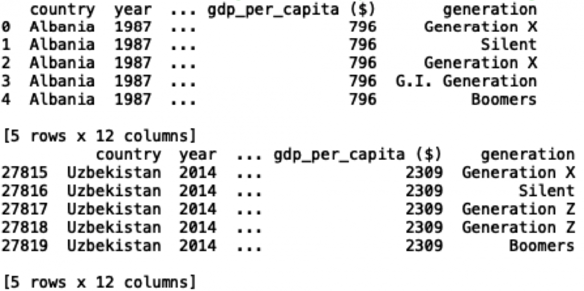
In python, if your dataset is in CSV file format, it reads using predefined functions. Reading and displaying data from the CSV file is as follows:
curDir = os.getcwd()
data=pd.read_csv(curDir + '/master.csv')
print(data.head())
print(data.tail())

print(data.sample(5))
print(data.sample(frac=0.1))
Another way of showing your data or displaying your data is as follows:
print(data.iloc[:,1:5].describe())
print(data.info())
print(data.columns)
#renaming data.
data=data.rename(columns={'country':'Country','year':'Year','sex':'Gender','age':'Age','suicides_no':'SuicidesNo','population':'Population','suicides/100k pop':'Suicides 100k Population','country-year':'CountryYear','HDI for year':'HDIForYear',' gdp_for_year ($) ':'GdpForYearMoney','gdp_per_capita ($)':'Gdp_Per_Capita','generation':'Generation'})
print(data.columns)
print(data.isnull().any())
print(data.isnull().values.any())
print(data.isnull().sum())
Simple Linear Regression Algorithm
In this example, I’m using a simple linear regression between GDP per Capital and Population. To begin with, as you can see in the graph, Gender was also included in the analysis. Below is the code implemented in Python.
sns.lmplot(x="Population", y="Gdp_Per_Capita", hue="Gender", data=data, palette="Set1")
plt.show()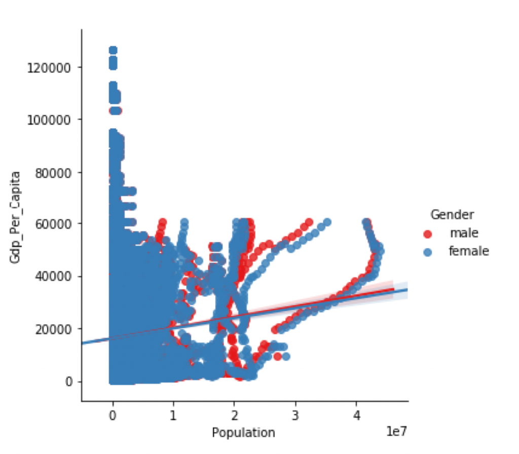
Data Visualization
There are so many ways you can show your data but as for my own preference, showing relevant data in a form of graph would be best emphasize. Python has a good way to represent it, so here’s how!
First, the graph represents the population of suicide rates in this presentation, it uses a simple scatterplot graph. Here’s how to implement scatterplot in python.
plt.figure(figsize=(10,10))
sns.stripplot(x="Year",y='Suicides 100k Population',data=data, palette="Set1")

plt.xticks(rotation=45)

plt.show()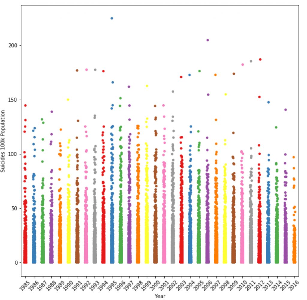
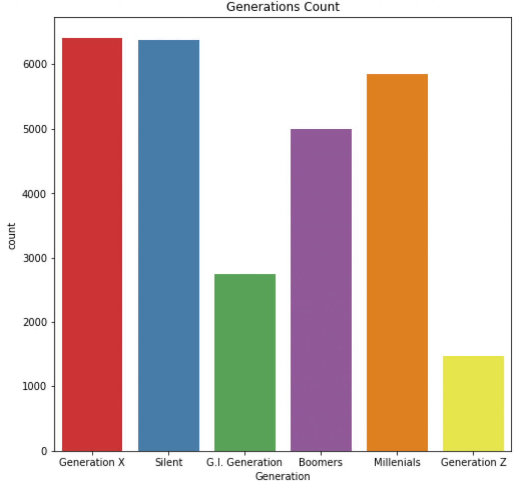
Second and finally the last graph have the same values to represent but for educational purposes, It represents both Pie graph and Bar graph. Check how python code differs in these data.
f,ax=plt.subplots(1,2,figsize=(18,8))
data['Generation'].value_counts().plot.pie(explode=[0.1,0.1,0.1,0.1,0.1,0.1],autopct='%1.1f%%',ax=ax[0],shadow=True)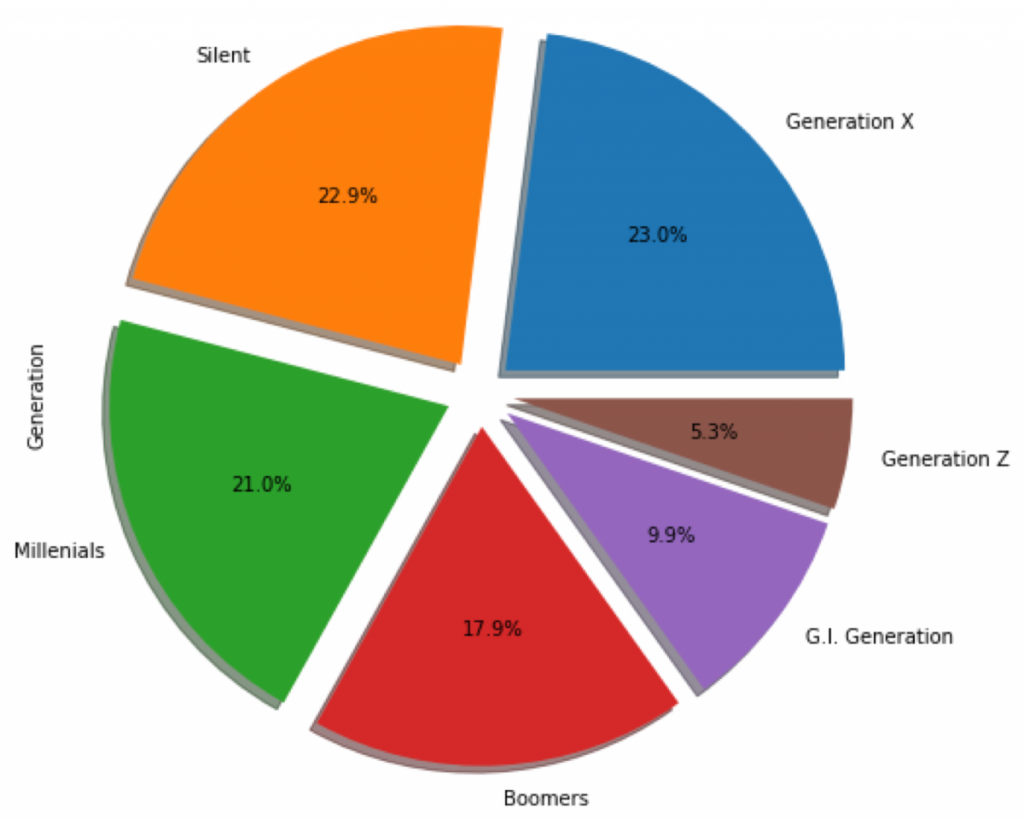
f,ax=plt.subplots(1,2,figsize=(18,8))
ax[0].set_title('Generations Summary')
ax[0].set_ylabel('Count')
sns.countplot('Generation',data=data,ax=ax[1], palette="Set1")
ax[1].set_title('Generations Count')
plt.show()
Here’s the entire code implementation in Python:
#!/usr/bin/env python3
#!/usr/bin/env python3
# -*- coding: utf-8 -*-
"""
Created on Mon Nov  4 13:42:48 2019

@author: juliet mendez

 - Mental Health Evaluation
 - Data from www.kaggle.com


"""

import numpy as np
import pandas as pd
import matplotlib.pyplot as plt
import seaborn as sns
import os

curDir = os.getcwd()
data=pd.read_csv(curDir + '/master.csv')
print(data.head())
print(data.tail())

print(data.sample(5))
print(data.sample(frac=0.1))


data=data.rename(columns={'country':'Country','year':'Year','sex':'Gender','age':'Age','suicides_no':'SuicidesNo','population':'Population','suicides/100k pop':'Suicides 100k Population','country-year':'CountryYear','HDI for year':'HDIForYear',' gdp_for_year ($) ':'GdpForYearMoney','gdp_per_capita ($)':'Gdp_Per_Capita','generation':'Generation'})

print(data.isnull().any())
print(data.isnull().values.any())

print(data.isnull().sum())

print("\n \n \n")

sns.lmplot(x="Population", y="Gdp_Per_Capita", hue="Gender", data=data, palette="Set1")
plt.show()
print("\n \n \n")
plt.figure(figsize=(10,10))
sns.stripplot(x="Year",y='Suicides 100k Population',data=data, palette="Set1")
plt.xticks(rotation=45)
plt.show()
print("\n \n \n")
data=data.drop(['HDIForYear','CountryYear'],axis=1)

min_year=min(data.Year)
max_year=max(data.Year)
print('Min Year :',min_year)
print('Max Year :',max_year)

data_country=data[(data['Year']==min_year)]

print("\n \n \n")
f,ax=plt.subplots(1,2,figsize=(18,8))
#pie chart
data['Generation'].value_counts().plot.pie(explode=[0.1,0.1,0.1,0.1,0.1,0.1],autopct='%1.1f%%',ax=ax[0],shadow=True)

#bar graph
ax[0].set_title('Generations Summary')
ax[0].set_ylabel('Count')
sns.countplot('Generation',data=data,ax=ax[1], palette="Set1")
ax[1].set_title('Generations Count')
plt.show()